Validity tests¶

Driving cycle, velocity and acceleration¶

Beside custom driving cycles, there are eleven default driving cycles to select from:

WLTC
WLTC 3.1
WLTC 3.2
WLTC 3.3
WLTC 3.4
CADC Urban
CADC Road
CADC Motorway
CADC Motorway 130
CADC
NEDC

They are needed to calculate a number of things, such as: * velocity, driving distance, driving time, and acceleration, * but also hot pollutant and noise emissions.

Manually, such parameters can be obtained the following way:

import pandas as pd
import numpy as np
# Retrieve the driving cycle WLTC 3 from the UNECE
driving_cycle = pd.read_excel('http://www.unece.org/fileadmin/DAM/trans/doc/2012/wp29grpe/WLTP-DHC-12-07e.xls',
            sheet_name='WLTC_class_3', skiprows=6, usecols=[2,4,5])

# Calculate velocity (km/h -> m/s)
velocity = driving_cycle['km/h'].values * 1000 / 3600

# Retrieve driving distance (-> km)
driving_distance = velocity.sum() * 1000

# Retrieve driving time (-> s)
driving_time = len(driving_cycle.values)

# Retrieve acceleration by calculating the delta of velocity per time interval of 2 seconds
acceleration = np.zeros_like(velocity)
acceleration[1:-1] = (velocity[2:] - velocity[:-2])/2

Using carculator, these parameters can be obtained the following way:

from carculator.energy_consumption import EnergyConsumptionModel
ecm = EnergyConsumptionModel('WLTC')

# Access the driving distance
ecm.velocity.sum() * 1000

# Access the driving time
len(ecm.velocity)

# Access the acceleration
ecm.acceleration

Both approaches should return identical results:

print(np.array_equal(velocity, ecm.velocity))
print(driving_distance == ecm.velocity.sum()*1000)
print(driving_time == len(ecm.velocity))
print(np.array_equal(acceleration, ecm.acceleration))

True
True
True
True

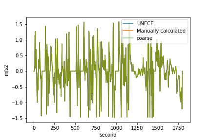
And the acceleration returned by carculator should equal the values given by the UNECE:

np.array_equal(np.around(ecm.acceleration,4),np.around(driving_cycle['m/s²'].values,4))

True

Which can be also be verified visually:

plt.plot(driving_cycle['m/s²'].values, label='UNECE')
plt.plot(acceleration, label='Manually calculated')
plt.plot(ecm.acceleration, label='carculator', alpha=0.6)
plt.legend()
plt.ylabel('m/s2')
plt.xlabel('second')
plt.savefig('comparison_driving_cycle.png')
plt.show()

Car and components masses¶

CarModel sizes and “builds” the vehicles. The vehicles attributes are accessed in the array attribute of the CarModel class. Filters like vehicle size class, year of manufacture and powertrain technology are convenient to use. A relevant calculated parameter is the driving mass, as it is determinant for the energy required to overcome rolling resistance, the drag, but also the energy required to move the vehicle over a given distance – kinetic energy, which is altogether defined as the tank to wheel energy, stored under the parameter TtW_energy.

Parameters such as total cargo mass, curb mass and driving mass, can be obtained the following way, for a 2020 battery electric SUV:

cm.array.sel(size='SUV', powertrain='BEV', year=2020, parameter=['cargo mass','curb mass', 'driving mass']).values

array([[  20.        ],
   [1719.56033224],
   [1874.56033224]])

One can check whether total cargo mass is indeed equal to cargo mass plus the product of the number of passengers and the average passenger weight:

total_cargo, cargo, passengers, passengers_weight = cm.array.sel(size='SUV', powertrain='BEV', year=2020,
    parameter=['total cargo mass','cargo mass','average passengers', 'average passenger mass']).values
print('Total cargo of {} kg, with a cargo mass of {} kg, and {} passengers of individual weight of {} kg.'.format(total_cargo[0], cargo[0], passengers[0], passengers_weight[0]))
print(total_cargo == cargo+(passengers * passengers_weight))

Total cargo of 155.0 kg, with a cargo mass of 20.0 kg, and 1.8 passengers of individual weight of 75.0 kg.
[True]

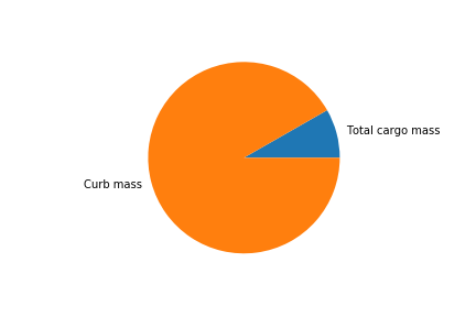
However, most of the driving mass is explained by the curb mass:

plt.pie(np.squeeze(cm.array.sel(size='SUV', powertrain='BEV', year=2020,
    parameter=['total cargo mass', 'curb mass']).values).tolist(), labels=['Total cargo mass', 'Curb mass'])
plt.show()

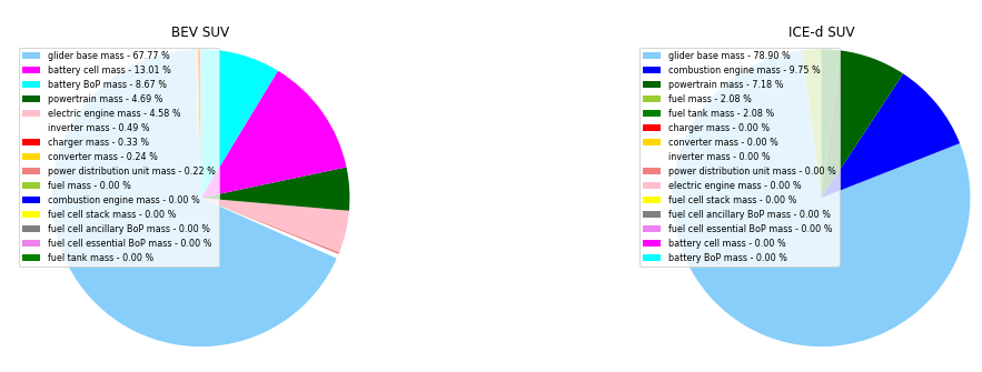
Here is a split between the components making up for the curb mass. One can see that, in the case of a battery electric SUV, most of the weight comes from the glider as well as the battery cells. On an equivalent diesel powertrain, the mass of the glider base is comparatively more important:

l_param=["fuel mass","charger mass","converter mass","glider base mass","inverter mass","power distribution unit mass",
        "combustion engine mass","electric engine mass","powertrain mass","fuel cell stack mass",
        "fuel cell ancillary BoP mass","fuel cell essential BoP mass","battery cell mass","battery BoP mass","fuel tank mass"]


colors = ['yellowgreen','red','gold','lightskyblue','white','lightcoral','blue','pink', 'darkgreen','yellow','grey','violet','magenta','cyan', 'green']

BEV_mass = np.squeeze(cm.array.sel(size='SUV', powertrain='BEV', year=2020,
        parameter=l_param).values)

percent = 100.*BEV_mass/BEV_mass.sum()

f = plt.figure(figsize=(15,10))

ax = f.add_subplot(121)

patches, texts = ax.pie(BEV_mass, colors=colors, startangle=90, radius=1.2)
ax.set_title('BEV SUV')
labels = ['{0} - {1:1.2f} %'.format(i,j) for i,j in zip(l_param, percent)]

sort_legend = True
if sort_legend:
    patches, labels, dummy =  zip(*sorted(zip(patches, labels, BEV_mass),
                                          key=lambda x: x[2],
                                          reverse=True))

ax.legend(patches, labels, loc='upper left', bbox_to_anchor=(-0.1, 1.),
           fontsize=8)


ICEV_d_mass = np.squeeze(cm.array.sel(size='SUV', powertrain='ICEV-d', year=2020,
        parameter=l_param).values)
percent = 100.*ICEV_d_mass/ICEV_d_mass.sum()

ax2 = f.add_subplot(122)

patches, texts = ax2.pie(ICEV_d_mass, colors=colors, startangle=90, radius=1.2)
ax2.set_title('ICE-d SUV')
labels = ['{0} - {1:1.2f} %'.format(i,j) for i,j in zip(l_param, percent)]

sort_legend = True
if sort_legend:
    patches, labels, dummy =  zip(*sorted(zip(patches, labels, ICEV_d_mass),
                                          key=lambda x: x[2],
                                          reverse=True))

ax2.legend(patches, labels, loc='upper left', bbox_to_anchor=(-0.1, 1.),
           fontsize=8)

plt.subplots_adjust(wspace=1)
plt.show()

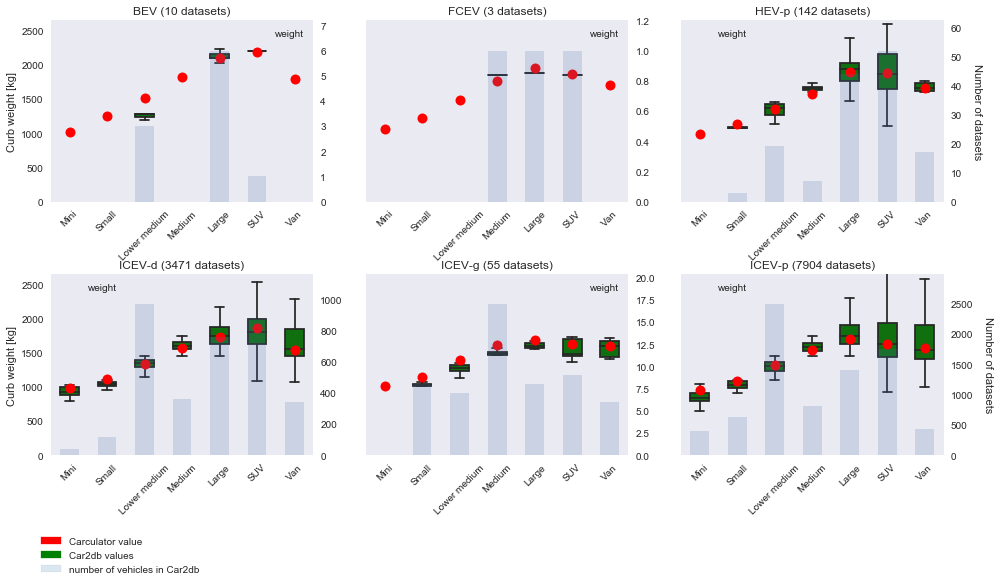
The curb mass returned by carculator for the year 2010 and 2020 is further calibrated against manufacturers’ data, per vehicle size class and powertrain technology. For example, we use the car database Car2db (https://car2db.com/) and load all the vehicles produced between 2015 and 2019 (11,500+ vehicles) to do the curb mass calibration for 2020 vehicles. The same exercise is done with vehicles between 2008 and 2012 to calibrate the curb mass of given by carculator for vehicles in 2010.