Using Carculator
Static vs. Stochastic mode
Note
Many examples are given in this example notebook that you can run directly on your computer.
The inventories can be calculated using the most likely value of the given input parameters (“static” mode), but also using randomly-generated values based on a probability distribution for those (“stochastic” mode).
For example, the drivetrain efficiency of SUVs in 2020, regardless of the powertrain, is given the most likely value (i.e., the mode) of 0.38, but with a triangular probability distribution with a minimum and maximum of 0.3 and 0.4, respectively.
Creating car models in static mode will use the most likely value of the given parameters to dimension the cars, etc., such as:
from carculator import *
cip = VehicleInputParameters()
cip.static()
dcts, array = fill_xarray_from_input_parameters(cip)
cm = CarModel(array)
cm.set_all()
Alternatively, if one wishes to work with probability distributions as parameter values instead:
from carculator import *
cip = VehicleInputParameters()
cip.stochastic(800)
dcts, array = fill_xarray_from_input_parameters(cip)
cm = CarModel(array)
cm.set_all()
This effectively creates 800 iterations of the same car models, picking pseudo-random value for the given parameters, within the probability distributions defined. This allows to assess later the effect of uncertainty propagation on characterized results.
In both case, a CarModel object is returned, with a 4-dimensional array array to store the generated parameters values, with the following dimensions:
- Vehicle sizes (called “size”):
Mini
Small
Lower medium
Medium
Large
SUV
Van
- Powertrains:
ICEV-p, ICEV-d, ICEV-g: vehicles with internal combustion engines running on gasoline, diesel and compressed gas, respectively.
HEV-p, HEV-d: vehicles with internal combustion engines running on gasoline and diesel, assisted with an electric engine.
PHEV-p, PHEV-d: vehicles with internal combustion engines running on gasoline and diesel, assisted with a plugin electric engine.
BEV: battery electric vehicles.
FCEV: fuel cell electric vehicles.
Year. Anything between 2000 and 2050.
Iteration number (length = 1 if static(), otherwise length = number of iterations).
cm.set_all() generates a CarModel object and calculates the energy consumption, components mass, as well as
exhaust and non-exhaust emissions for all vehicle profiles.
Custom values for given parameters
You can pass your own values for the given parameters, effectively overriding the default values.
For example, you may think that the base mass of the glider for large diesel and petrol cars is 1600 kg in 2020 and 1,500 kg in 2040, and not 1,500 kg as defined by the default values. It is easy to change this value. You need to create first a dictionary and define your new values as well as a probability distribution if needed :
dic_param = {
('Glider', ['ICEV-d', 'ICEV-p'], 'Large', 'glider base mass', 'triangular'): {(2020, 'loc'): 1600.0,
                                                             (2020, 'minimum'): 1500.0,
                                                             (2020, 'maximum'): 2000.0,
                                                             (2040, 'loc'): 1500.0,
                                                             (2040, 'minimum'): 1300.0,
                                                             (2040, 'maximum'): 1700.0}}
Then, you simply pass this dictionary to modify_xarray_from_custom_parameters(<dic_param or filepath>, array), like so:
cip = VehicleInputParameters()
cip.static()
dcts, array = fill_xarray_from_input_parameters(cip)
modify_xarray_from_custom_parameters(dic_param, array)
cm = CarModel(array, cycle='WLTC')
cm.set_all()
Alternatively, instead of a Python dictionary, you can pass a file path pointing to an Excel spreadsheet that contains
the values to change, following this template.
The following probability distributions are accepted: * “triangular” * “lognormal” * “normal” * “uniform” * “none”
Inter and extrapolation of parameters
carculator creates by default car models for the year 2000, 2010, 2020 and 2040.
It is possible to inter and extrapolate all the parameters to other years simply by writing:
array = array.interp(year=[2018, 2022, 2035, 2040, 2045, 2050], kwargs={'fill_value': 'extrapolate'})
However, we do not recommend extrapolating for years before 2000 or beyond 2050.
Changing the driving cycle
carculator gives the user the possibility to choose between several driving cycles. Driving cycles are determinant in
many aspects of the car model: hot pollutant emissions, noise emissions, tank-to-wheel energy, etc. Hence, each driving
cycle leads to slightly different results. By default, if no driving cycle is specified, the WLTC driving cycle is used.
To specify a driving cycle, simply do:
cip = VehicleInputParameters()
cip.static()
dcts, array = fill_xarray_from_input_parameters(cip)
cm = CarModel(array, cycle='WLTC 3.4')
cm.set_all()
In this case, the driving cycle WLTC 3.4 is chosen (this driving cycle is in fact a sub-part of the WLTC driving cycle, mostly concerned with driving on the motorway at speeds above 80 km/h). Driving cycles currently available:
WLTC
WLTC 3.1
WLTC 3.2
WLTC 3.3
WLTC 3.4
CADC Urban
CADC Road
CADC Motorway
CADC Motorway 130
CADC
NEDC
The user can also create custom driving cycles and pass it to the CarModel class:
import numpy as np
x = np.linspace(1, 1000)
def f(x):
    return np.sin(x) + np.random.normal(scale=20, size=len(x)) + 70

cycle = f(x)
cm = CarModel(array, cycle=cycle)
Accessing calculated parameters of the car model
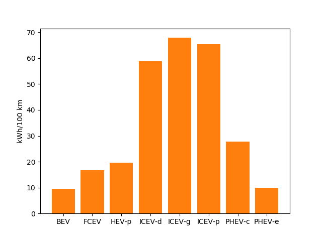
Hence, the tank-to-wheel energy requirement per km driven per powertrain technology for a SUV in 2020 can be obtained from the CarModel object:
TtW_energy = cm.array.sel(size='SUV', year=2020, parameter='TtW energy', value=0) * 1/3600 * 100

plt.bar(TtW_energy.powertrain, TtW_energy)
plt.ylabel('kWh/100 km')
plt.show()
Note
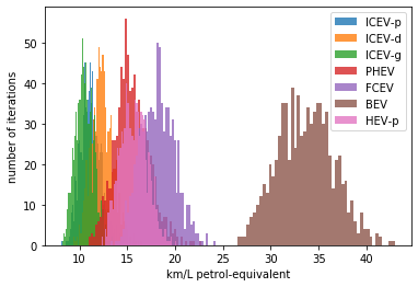
If you call the stochastic() method of the VehicleInputParameters, you would have several values stored for a given calculated parameter
in the array. The number of values correspond to the number of iterations you passed to stochastic().
For example, if you ran the model in stochastic mode with 800 iterations as shown in the section above, instead of one value for the tank-to-wheel energy, you would have a distribution of values:
l_powertrains = TtW_energy.powertrain
[plt.hist(e, bins=50, alpha=.8, label=e.powertrain.values) for e in TtW_energy]
plt.ylabel('kWh/100 km')
plt.legend()
Any other attributes of the CarModel class can be obtained in a similar way. Hence, the following code lists all direct exhaust emissions included in the inventory of an petrol Van in 2020:
List of all the given and calculated parameters of the car model:
list_param = cm.array.coords['parameter'].values.tolist()
Return the parameters concerned with direct exhaust emissions (we remove noise emissions):
direct_emissions = [x for x in list_param if 'emission' in x and 'noise' not in x]
Finally, return their values and display the first 10 in a table:
cm.array.sel(parameter=direct_emissions, year=2020, size='Van', powertrain='BEV').to_dataframe(name='direct emissions')
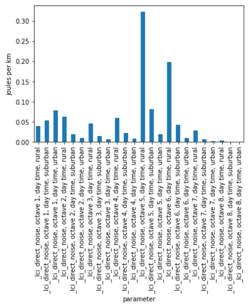
Or we could be interested in visualizing the distribution of non-characterized noise emissions, in joules:
noise_emissions = [x for x in list_param if 'noise' in x]
data = cm.array.sel(parameter=noise_emissions, year=2020, size='Van', powertrain='ICEV-p', value=0)\
    .to_dataframe(name='noise emissions')['noise emissions']
data[data>0].plot(kind='bar')
plt.ylabel('joules per km')
Modify calculated parameters
As input parameters, calculated parameters can also be overridden. For example here, we override the driving mass of large diesel vehicles for 2010 and 2020:
cm.array.loc['Large','ICEV-d', 'driving mass', [2010, 2020]] = [[2000],[2200]]
Characterization of inventories (static)
carculator makes the characterization of inventories easy. You can characterize the inventories directly from
carculator against midpoint impact assessment methods.
For example, to obtain characterized results against the midpoint impact assessment method ReCiPe for all cars:
ic = InventoryCalculation(cm)
results = ic.calculate_impacts()
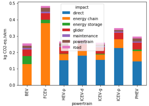
Hence, to plot the carbon footprint for all medium cars in 2020:
results.sel(size='Medium', year=2020, impact_category='climate change', value=0).to_dataframe('impact').unstack(level=1)['impact'].plot(kind='bar',
            stacked=True)
plt.ylabel('kg CO2-eq./vkm')
plt.show()
Note
For now, only the ReCiPe method is available for midpoint characterization. Also, once the instance of the CarModel
class has been created, there is no need to re-create it in order to calculate additional environmental impacts (unless you wish to
change values of certain input or calculated parameters, the driving cycle or go from static to stochastic mode).
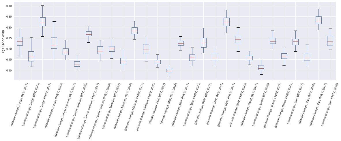
Characterization of inventories (stochastic)
In the same manner, you can obtain distributions of results, instead of one-point values if you have run the model in stochastic mode (with 500 iterations and the driving cycle WLTC).
cip = VehicleInputParameters()
cip.stochastic(500)
dcts, array = fill_xarray_from_input_parameters(cip)
cm = CarModel(array, cycle='WLTC')
cm.set_all()
scope = {
    'powertrain':['BEV', 'PHEV'],
}
ic = InventoryCalculation(cm, scope=scope)

results = ic.calculate_impacts()

data_MC = results.sel(impact_category='climate change').sum(axis=3).to_dataframe('climate change')
plt.style.use('seaborn')
data_MC.unstack(level=[0,1,2]).boxplot(showfliers=False, figsize=(20,5))
plt.xticks(rotation=70)
plt.ylabel('kg CO2-eq./vkm')
Many other examples are described in a Jupyter Notebook in the examples folder.
Export of inventories (static)
- Inventories can be exported as:
a Python list of exchanges
a Brightway2 bw2io.importers.base_lci.LCIImporter object, ready to be imported in a Brigthway2 environment
an Excel file, to be imported in a Brigthway2 environment
a CSV file, to be imported in SimaPro 9.x.
ic = InventoryCalculation(cm)

# export the inventories as a Python list
mylist = ic.export_lci()
# export the inventories as a Brightway2 object
import_object = ic.export_lci_to_bw()
# export the inventories as an Excel file (returns the file path of the created file)
filepath = ic.export_lci_to_excel(software_compatibility="brightway2", ecoinvent_version="3.7")
filepath = ic.export_lci_to_excel(software_compatibility="simapro", ecoinvent_version="3.6")
Export of inventories (stochastic)
If you had run the model in stochastic mode, the export functions return in addition an array that contains pre-sampled values for each parameter of each car, in order to perform Monte Carlo analyses in Brightway2.
ic = InventoryCalculation(cm)

# export the inventories as a Python list
mylist, presamples_arr = ic.export_lci()
# export the inventories as a Brightway2 object
import_object, presamples_arr = ic.export_lci_to_bw()
# export the inventories as an Excel file (note that this method does not return the presamples array)
filepath = ic.export_lci_to_excel()
Import of inventories (static)
The background inventory is originally a combination between ecoinvent 3.6 and outputs from PIK’s REMIND model. Outputs from PIK’s REMIND are used to project expected progress in different sectors into ecoinvent. For example, the efficiency of electricity-producing technologies as well as the electricity mixes in the future for the main world regions are built upon REMIND outputs. The library used to create hybrid versions of the ecoinvent database from PIK’s REMIND is called premise. This means that, as it is, the inventory cannot properly link to ecoinvent 3.6 or 3.7 unless some transformation is performed before. These transformations are in fact performed when exporting the inventory. Hence, when doing:
ic.export_lci_to_excel(ecoinvent_compatibility=True, ecoinvent_version="3.6")
the resulting inventory should properly link to the unmodified version of ecoinvent 3.6 cutoff. Should you wish to export an inventory to link with a IAM-modified version of ecoinvent, just export the inventory with the ecoinvent_compatibility argument set to False.
ic.export_lci_to_excel(ecoinvent_compatibility=False, ecoinvent_version="3.6")
In that case, the inventory will only link to a custom ecoinvent database produced by premise.
But in any case, the following script should successfully import the inventory into a Brightway2 project:
import brightway2 as bw
bw.projects.set_current("test_carculator")
import bw2io
fp = r"C:\file_path_to_the_inventory\lci-test.xlsx"

i = bw2io.ExcelImporter(fp)
i.apply_strategies()

i.match_database("name_of_the_ecoinvent_db", fields=('name', 'unit', 'location', 'reference product'))
i.match_database("biosphere3", fields=('name', 'unit', 'categories'))
i.match_database("additional_biosphere", fields=('name', 'unit', 'categories'))
i.match_database(fields=('name', 'unit', 'location'))

i.statistics()

# if there are some unlinked left
i.add_unlinked_flows_to_biosphere_database()

i.write_database()