Modeling
This document describes the carculator model, assumptions
and inventories as exhaustively as possible.
carculator is an open-source Python library. Its code is publicly
available via its Github
repository.
You can also download an examples notebook, that guides new users into performing life cycle analyses.
Finally, there
is also an online graphical user interface available at
https://carculator.psi.ch.
Overview of carculator modules
The main module model.py builds
the vehicles and delegates the calculation of motive and auxiliary
energy, noise, abrasion and exhaust emissions to satellite modules. Once
the vehicles are fully characterized, the set of calculated parameters
are passed to inventory.py which derives life cycle inventories and
calculates life cycle impact indicators. Eventually, these inventories
can be passed to export.py to be exported to various LCA software.
Vehicle modelling
The modelling of vehicles along powertrain types, time and size classes is described in this section. It is also referred to as foreground modelling.
Size classes
Originally, carculator defines nine size classes, namely: Micro, Mini,
Small, Lower medium, Medium, Large, Medium SUV, Large SUV and Van,
according to the following criteria, adapted from the work of [Christian and others, 2014] and
shown in Table 1.
EU segment |
EU segment definition |
carculator |
Minimum footprint [m2] |
Maximum footprint [m2] |
Minimum curb mass [kg] |
Maximum curb mass [kg] |
Examples |
|---|---|---|---|---|---|---|---|
L7e |
Micro cars/Heavy quadricycles |
Micro |
400 |
600 |
Renault Twizzy, Microlino |
||
A |
Mini cars |
Mini |
3.4 |
1050 |
Renault Twingo, Smart ForTwo, Toyota Aygo |
||
B |
Small cars |
Small |
3.4 |
3.8 |
900 |
1’100 |
Renault Clio, VW Polo, Toyota Yaris |
C |
Medium cars |
Lower medium |
3.8 |
4.3 |
1’250 |
1’500 |
VW Golf, Ford Focus, Mercedes Class A |
C |
Medium |
3.9 |
4.4 |
1’500 |
1’750 |
VW Passat, Audi A4, Mercedes Class C |
|
D |
Large/Executive |
Large |
4.4 |
1’450 |
2’000 |
Tesla Model 3, BMW 5 Series, Mercedes E series |
|
J |
Sport Utility |
Medium SUV |
4.5 |
1’300 |
2’000 |
Toyota RAV4, Peugeot 2008, Dacia Duster |
|
J |
Sport Utility |
Large SUV |
6 |
2’000 |
2’500 |
Audi Q7, BMW X7, Mercedes-Benz GLS, Toyota Landcruiser, Jaguar f-Pace |
|
M |
Multi-Purpose Vehicles |
Van |
Defined by body type rather than mass and footprint. |
VW Transporter, Mercedes Sprinter, Ford Transit |
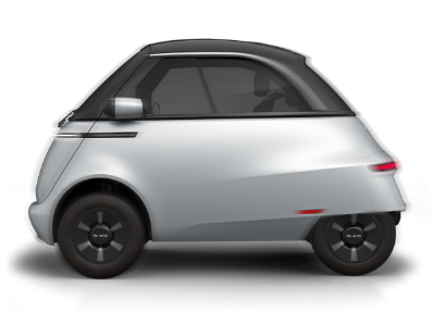
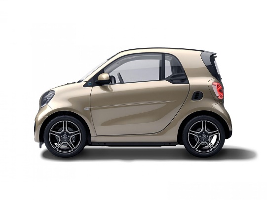
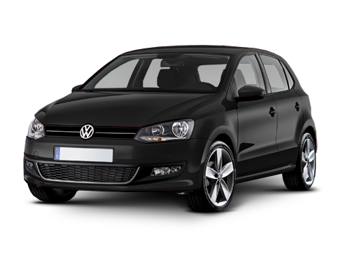
Example of Micro car (Microlino), Mini car (Smart) and Small/Compact car (VW Polo)
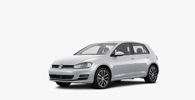
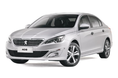
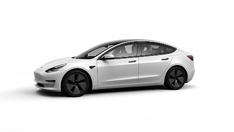
Example of Lower medium car (VW Golf), Medium car (Peugeot 408) and Large car (Tesla Model 3)
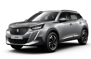
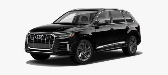

Example of Medium SUV car (Peugeot 2008), Large SUV car (Audi Q7) and Van (Fiat Ducato)
Note
Important remark: Micro cars are not considered passenger cars in the Swiss and European legislation, but heavy quadricycles. We do however assimilate them to passenger cars. They are only modelled with a battery electric powertrain.
Note
Important remark: Sport Utility Vehicles (SUV) are considered more as a body type than a size class. These vehicles have distinct aerodynamic properties, but their curb mass can be as light as that of a VW Polo or a Renault Clio (i.e., the Dacia Duster or Peugeot 2008 have a curb mass of 1’150 kg, against 1’100-1’300 kg for a VW Polo) or as heavy as a Mercedes Class E (i.e., the Audi Q7 has a minimum curb mass of 2’000 kg, against 1’900 kg for a Mercedes Class E). To assess the impacts of very large SUV, the “Large SUV” category has been added, to represent SUV models with a very high curb mass (2’000 kg and above) and footprint.
Manufacture year and emission standard
Several emission standards are considered. For simplicity, it is assumed that the vehicle manufacture year corresponds to the registration year, as shown in Table 2.
Start of registration |
End of registration (incl.) |
Manufacture
year in
|
|
|---|---|---|---|
EURO-3 |
2001 |
2005 |
2003 |
EURO-4 |
2006 |
2010 |
2008 |
EURO-5 |
2011 |
2014 |
2013 |
EURO-6 a/b |
2015 |
2017 |
2016 |
EURO-6 c |
2018 |
2018 |
2018 |
EURO-6 d (temp) |
2019 |
2020 |
2019 |
EURO-6 d |
2021 |
2021 |
|
EURO-7 |
2026 |
Size and mass-related parameters and modeling
The vehicle glider and its components (powertrain, energy storage, etc.) are sized according to engine power, which itself is conditioned by the curb mass of the vehicle. The curb mass of the vehicle is the sum of the vehicle components (excluding the driver and possible cargo) as represented in Figure 1.
Figure 1: Vehicle mass calculation workflow
This is an iterative process that stops when the curb mass of the vehicle converges, as illustrated in Figure 2.
Figure 2: Representation of the convergence of the sizing of the passenger car model
Curb mass of the vehicle
This function calculates and sets the vehicle’s mass properties:
Curb mass: The mass of the vehicle and fuel, without people or cargo. Total cargo mass: The mass of the cargo and passengers. Driving mass: The sum of the curb mass and total cargo mass.
Function steps: 1. Set the curb mass as the product of the glider base mass and (1 - lightweighting). 2. Create a list of mass components to be included in the curb mass calculation. 3. Add the sum of these mass components to the curb mass. 4. If a target mass is provided, override the vehicle mass with the target mass. 5. Calculate the total cargo mass by summing the product of average passengers and average passenger mass, and the cargo mass. 6. Calculate the driving mass by adding the curb mass and total cargo mass.
With:
\(m_{curb}\) being the vehicle curb mass, in kg
\(m_{fuel}\) being the fuel mass, in kg
\(m_{charger}\) being the electric onboard charge mass, in kg
\(m_{conv}\) being the current converter, in kg
\(m_{inv}\) being the current AC/DC inverter, in kg
\(m_{distr}\) being the power distribution unit, in kg
\(m_{comb}\) being the combustion engine mass, in kg
\(m_{elec}\) being the electric motor mass, in kg
\(m_{pwt}\) being the powertrain mass, in kg
\(m_{fcstack}\) being the fuel cell stack mass, in kg
\(m_{fcauxbop}\) being the fuel cell auxiliary components mass, in kg
\(m_{battcell}\) being the battery cell mass, in kg
\(m_{battbop}\) being the battery auxiliary components mass, in kg
\(m_{fcessbop}\) being the fuel cell essential components mass, in kg
\(m_{fueltank}\) being the fuel tank mass, in kg
For each iteration, the tank-to-wheel energy consumption (i.e., the motive energy minus any recuperated braking energy, together with the needed auxiliary energy to power onboard electronics) of the vehicle is calculated (i.e., to size the energy storage components, calculate the fuel consumption, etc.), as described later in this section.
Cargo and driving mass of the vehicle
The cargo mass of the vehicle is the sum of the cargo mass and the passenger mass.
Where:
\(m_{cargo}\) is the cargo mass, in kg,
and \(m_{passenger}\) is the passenger mass.
The driving mass of the vehicle is the sum of the curb mass and the cargo mass.
Where:
\(m_{curb}\) is the curb mass, in kg,
\(m_{cargo}\) is the cargo mass, in kg,
and \(m_{driving}\) is the driving mass, in kg.
Light-weight rates
Because the LCI dataset used to represent the glider of the vehicle is not representative of today’s’ use of light-weighting materials, such as aluminium (i.e., the dataset “glider for passenger cars” only contains 0.5% of its mass in aluminium) and advanced high strength steel (AHSS), an amount of such light-weighting materials is introduced to substitute conventional steel and thereby reduce the mass of the glider.
As further explained under the Curb mass calibration section, the mass of the glider is reduced by replacing steel with a mix of aluminium and AHSS. Hence, the amounts of light weighting materials introduced depend on the rate of glider light weighting in 2020 relative to 2000 (approximately 11% for combustion engine vehicles). The amount of aluminium introduced is further cross-checked with the amounts indicated in [Frontier, 2019] and listed in Table 3, and comes in addition to the aluminium already contained in the LCI datasets for the engine and transmission.
Note
Important remark: The light-weighting rate is for most vehicles approximately 11% in 2020 relative to 2000. However, battery-equipped vehicles are an exception to this: Medium, Large and Large SUV vehicles have significantly higher light weighting rates to partially compensate for the additional mass of their batteries. In order to match the battery capacity and the curb mass of their respective size class, their light weighting rate is increased to 14, 28 and 30%, respectively. This trend is also confirmed by [Frontier, 2019], showing that battery electric vehicles have 85% more aluminium than combustion engine vehicles, partly going into the battery management system, and partly going into the chassis to compensate for the extra mass represented by the battery.
These light-weighting rates have been fine adjusted to match the curb mass of a given size class, while preserving the battery capacity. For example, in the case of the Large SUV, its curb mass should approximately be 2’200 kg, with an 80 kWh battery weighting 660 kg (e.g., Jaguar i-Pace). This is possible with a 30% light weighting rate, introducing approximately 460 kg of aluminium in the chassis (which matches roughly with the value given for an Audi e-Tron in Table 3) and 1’008 kg of AHSS, in lieu of 2’034 kg of regular steel.
Used in source |
Basic |
Sub-Compact |
Compact |
Midsize |
Large |
Audi e-Tron |
||
|---|---|---|---|---|---|---|---|---|
Used in carculator |
Small |
Medium |
Large |
Large SUV (BEV) |
||||
Average aluminium content per vehicle [kg] |
77 |
98 |
152 |
266 |
442 |
804 |
||
Share of aluminium mass in components other than engine and transmission [%] |
66% |
|||||||
Aluminium to be added to the glider [%] |
65 |
175 |
292 |
530 |
Curb mass calibration
The final curb mass obtained for each vehicle is calibrated against the European Commission’s database for CO2 emission tests for passenger cars (hereafter called EC-CO2-PC) using the NEDC/WLTP driving cycles [Commission, 2021]. Each vehicle registered in the European Union is tested and several of the vehicle attributes are registered (e.g., dimension, curb mass, driving mass, CO2 emissions, etc.). This has represented about 15+ million vehicles per year for the past five years.
The figure below shows such calibration for the years 2010, 2013, 2016,
2018, 2019 and 2020 – to be representative of EURO-4, -5, 6 a/b, 6-c
and 6-d-temp vehicles. No measurements are available for 2003 (EURO-3)
or 2021 (EURO-6-d). After cleaning the data from the EC-CO2-PC database,
it represents 27 million points to calibrate the curb mass of the
vehicles with. Green vertical bars represent the span of 50% of the curb
mass distribution, and the red dots are the curb mass values modeled by
carculator.
Figure 3: Calibration of the curb mass of the passenger car model against the EC-CO2-PC database. Red dots: values modeled by carculator. Green box-and-whiskers: values distribution from the EC-CO2-PC database (box: 50% of the distribution, whiskers: 90% of the distribution). Micro cars are not represented in the EC-CO2-PC database. Sample size for each size class is given above each chart. M = Mini, S = Small, L-M = Lower medium, M = Medium, L = Large, L-SUV = Large SUV. Source for vehicle tank-to-wheel energy consumption measurements: [Agency, 2019].
Table 4 shows the mass distribution for gasoline and battery electric passenger cars resulting from the calibration. Mass information on other vehicles is available in the vehicles’ specifications spreadsheet. These numbers may change if the default input values (i.e., engine power, fuel tank size, etc.) are changed.
Gasoline |
Battery electric |
||||||||
|---|---|---|---|---|---|---|---|---|---|
in kilograms |
Small |
Medium |
Large |
Large SUV |
Micro |
Small |
Medium |
Large |
Large SUV |
Glider base mass |
998 |
1’170 |
1’550 |
1’900 |
350 |
998 |
1’170 |
1’550 |
1’900 |
Light weighting |
-110 |
-129 |
-171 |
-209 |
-35 |
-140 |
-164 |
-434 |
-570 |
Glider mass |
888 |
1’041 |
1’380 |
1’691 |
315 |
858 |
1’006 |
1’116 |
1’330 |
Powertrain mass |
96 |
106 |
132 |
140 |
42 |
67 |
77 |
94 |
100 |
Engine or motor mass |
111 |
125 |
157 |
168 |
29 |
61 |
73 |
96 |
102 |
Energy storage mass |
72 |
85 |
104 |
104 |
120 |
276 |
360 |
580 |
660 |
Electronics mass |
3 |
4 |
5 |
7 |
23 |
23 |
23 |
23 |
23 |
Curb mass |
1’170 |
1’361 |
1’777 |
2’110 |
529 |
1’285 |
1’540 |
1’910 |
2’215 |
Passenger mass |
120 |
120 |
120 |
120 |
120 |
120 |
120 |
120 |
120 |
Cargo mass |
20 |
20 |
20 |
20 |
20 |
20 |
20 |
20 |
20 |
Driving mass |
1’310 |
1’501 |
1’917 |
2’250 |
669 |
1’425 |
1’680 |
2’050 |
2’355 |
Energy consumption
The energy consumption model of carculator calculates the energy
required at the wheels by considering different types of resistance.
Some of these resistances are related to the vehicle size class. For
example, the frontal area of the vehicle influences the aerodynamic
drag. Also, the kinetic energy to overcome the vehicle’s inertia is
influenced by the mass of the vehicle (which partially correlates to
with the size class or body type), but also by the acceleration required
by the driving cycle. Other resistances, such as the climbing effort,
are instead determined by the driving cycle (but the vehicle mass also
plays a role here).
Here is how the different types of resistance are calculated:
Rolling resistance:
F_rolling (N) = driving_mass (kg) * rr_coef (dimensionless) * g (m/s^2) * (velocity (m/s) > 0)
Air resistance:
F_air (N) = 0.5 * rho_air (kg/m^3) * drag_coef (dimensionless) * frontal_area (m^2) * velocity^2 (m^2/s^2)
Gradient resistance:
F_gradient (N) = driving_mass (kg) * g (m/s^2) * sin(gradient (radians)) * (velocity (m/s) > 0)
Inertia:
F_inertia (N) = driving_mass (kg) * acceleration (m/s^2)
Total resistance:
F_total (N) = F_rolling (N) + F_air (N) + F_gradient (N) + F_inertia (N)
Motive energy at wheels:
E_wheels (J) = max(F_total (N), 0)
Motive energy:
E_motive (Wh) = E_wheels (J) / engine_efficiency (dimensionless) / transmission_efficiency (dimensionless) / fuel_cell_system_efficiency (dimensionless) * 2.778e-4 (Wh/J)
Recuperated energy:
F_rolling (N) = driving_mass (kg) * rr_coef (dimensionless) * g (m/s^2) * (velocity (m/s) > 0)
Auxiliary energy:
E_aux = aux_energy (Wh/km) = aux_power (W) + (p_cooling (W) / heat_pump_cop_cooling (dimensionless) * cooling_consumption (Wh/km)) + (p_heating (W) / heat_pump_cop_heating (dimensionless) * heating_consumption (Wh/km)) + p_battery_cooling (W) + p_battery_heating (W)
In this representation, E_motive represents the motive energy per kilometer driven, E_recuperated represents the energy recuperated per kilometer driven, and E_aux represents the auxiliary energy consumption per kilometer driven. The results are returned in kilojoules/km (kJ/km).
Once the energy required at the wheels is known, the model goes on to calculate the energy required at the tank level by considering additional losses along the drive train (i.e., axles, gearbox, and engine losses – see Engine and transmission efficiency). The different types of resistance considered are depicted in Figure 4, and the module calculation workflow is presented in Figure 5.
Powertrains that are partially or fully electrified have the possibility to recuperate a part of the energy spent for propulsion during deceleration or braking. The round-trip battery energy loss (which is the sum of the charge and discharge battery loss, described in Figure 4) is subtracted from the recuperated energy. For hybrid vehicles (i.e., HEV-p, HEV-d), this allows to downsize the combustion engine and improve the overall tank-to-wheel efficiency, as explained in [Brian and others, 2020].
Figure 4: Representation of the different types of resistance considered.
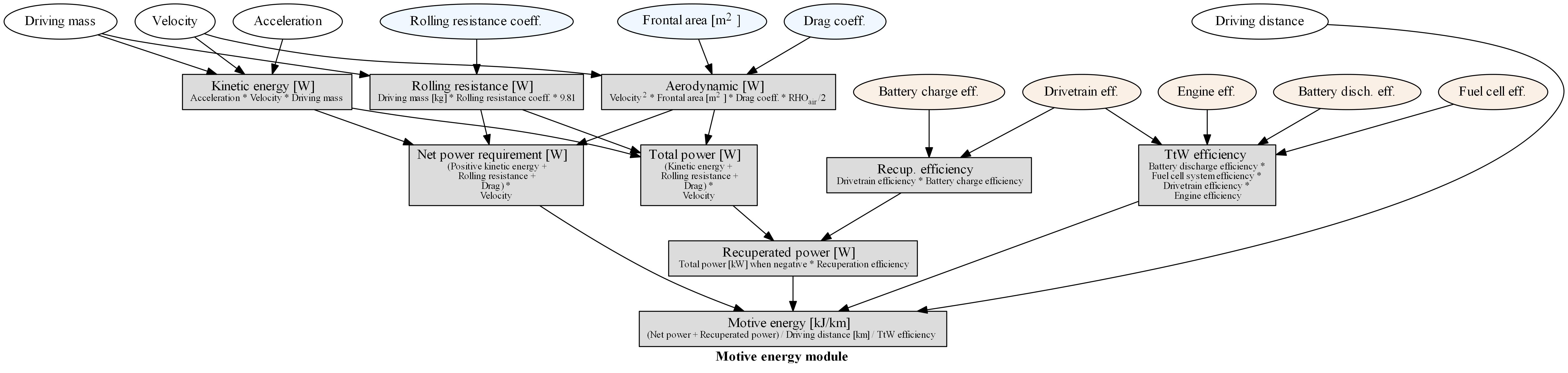
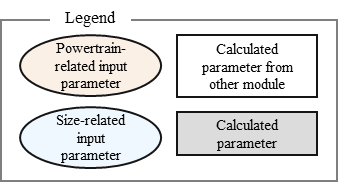
Figure 5: Motive energy calculation workflow
Finally, for each second of the driving cycle, the auxiliary power load is considered. It comprises an auxiliary base power load (i.e., to operate onboard electronics), as well as the power load from heating and cooling. While electric vehicles provide energy from the battery to supply heating and cooling (i.e., thereby decreasing the available energy available for traction), combustion vehicles recover enough waste engine heat to supply adequate heating. The values considered for the auxiliary base power load and for the power load for heating and cooling are presented in Table 5. These values are averaged over the whole year, based on maximum demand and share of operation.
Auxiliary power base demand [W] |
Heating power demand [W] |
Cooling power demand [W] |
|||||||||
|---|---|---|---|---|---|---|---|---|---|---|---|
Micro |
Small |
Medium |
Large |
Large SUV |
Micro |
Small |
Medium |
Large |
Large SUV |
||
ICEV, HEV, PHEV |
94 |
Provided by engine |
250 |
320 |
350 |
350 |
|||||
BEV, FCEV |
75 |
200 |
250 |
320 |
350 |
350 |
0 |
250 |
320 |
350 |
350 |
Where:
\(P_{base}\) is the auxiliary base power load [W],
\(P_{heating}\) is the power load for heating [W],
\(P_{cooling}\) is the power load for cooling [W],
\(D_{heating}\) is the demand for heating [0-1] (=0 for non-electric vehicles),
and \(D_{cooling}\) is the demand for cooling [0-1].
To convert it into an energy consumption \(F_{aux}\) [kj/km], the auxiliary power load is multiplied by the time of the driving cycle and divided by the distance driven:
Where: \(T\) is the driving cycle time [seconds] and D is the distance [m].
Note
Important remark: Micro cars are not equipped with an air conditioning system. Hence, their cooling energy requirement is set to zero.
A driving cycle is used to calculate the tank-to-wheel energy required by the vehicle to drive over one kilometer. For example, the WLTC driving cycle comprises a mix of urban, sub-urban and highway driving. It is assumed representative of average Swiss and European driving profile - although this would likely differ in the case of intensive mountain driving.
Figure 6 exemplifies such calculation for a medium battery electric passenger car manufactured in 2020, using the WLTC driving cycle.
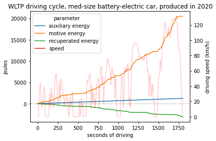
Figure 6: Cumulated tank-to-wheel energy consumption, along the WLTC driving cycle, for a mid-size battery electric vehicle from 2020
Figure 7: Driving cycle and related parameters
So, the tank-to-wheel energy consumption \(F_{ttw}\) is the sum of the motive energy and the energy required to power auxiliary equipment. It is calculated as:
Where:
\(F_{motive}\) is the motive energy,
and \(F_{aux}\) is the auxiliary energy.
There are no fuel consumption measurements available for fuel cell vehicles. Values found in the literature and from manufacturers data are used to approximate the engine and transmission efficiency and to calibrate the final energy consumption.
Engine and transmission efficiency
Engine and transmission efficiencies for the conventional gasoline, diesel and electric powertrains (including fuel cell electric powertrains) are defined as a function of the utilized engine power for each second of the driving cycle (i.e., the power load over the rated power output of the engine). Such relation is shown in Hjelkrem et al. 2020 [Hjelkrem et al., 2020]. Unfortunately, such relation is not given for compressed gas powertrains, which we assume to be 17.5% less efficient than diesle powertrains [JEC Well-to-Wheels report v5: Well-to-Wheels analysis of future automotive fuels and powertrains in the European context, 2020]. The specific values for engine and transmission efficiency in relation to utilized power can be consulted here . Hjelkrem et al. 2020 [Hjelkrem et al., 2020] only give the overall tank-to-wheel efficiency, which we decompose, assuming a static transmission efficiency and a varying engine efficiency (the product of which gives the tank-to-wheel efficiency).
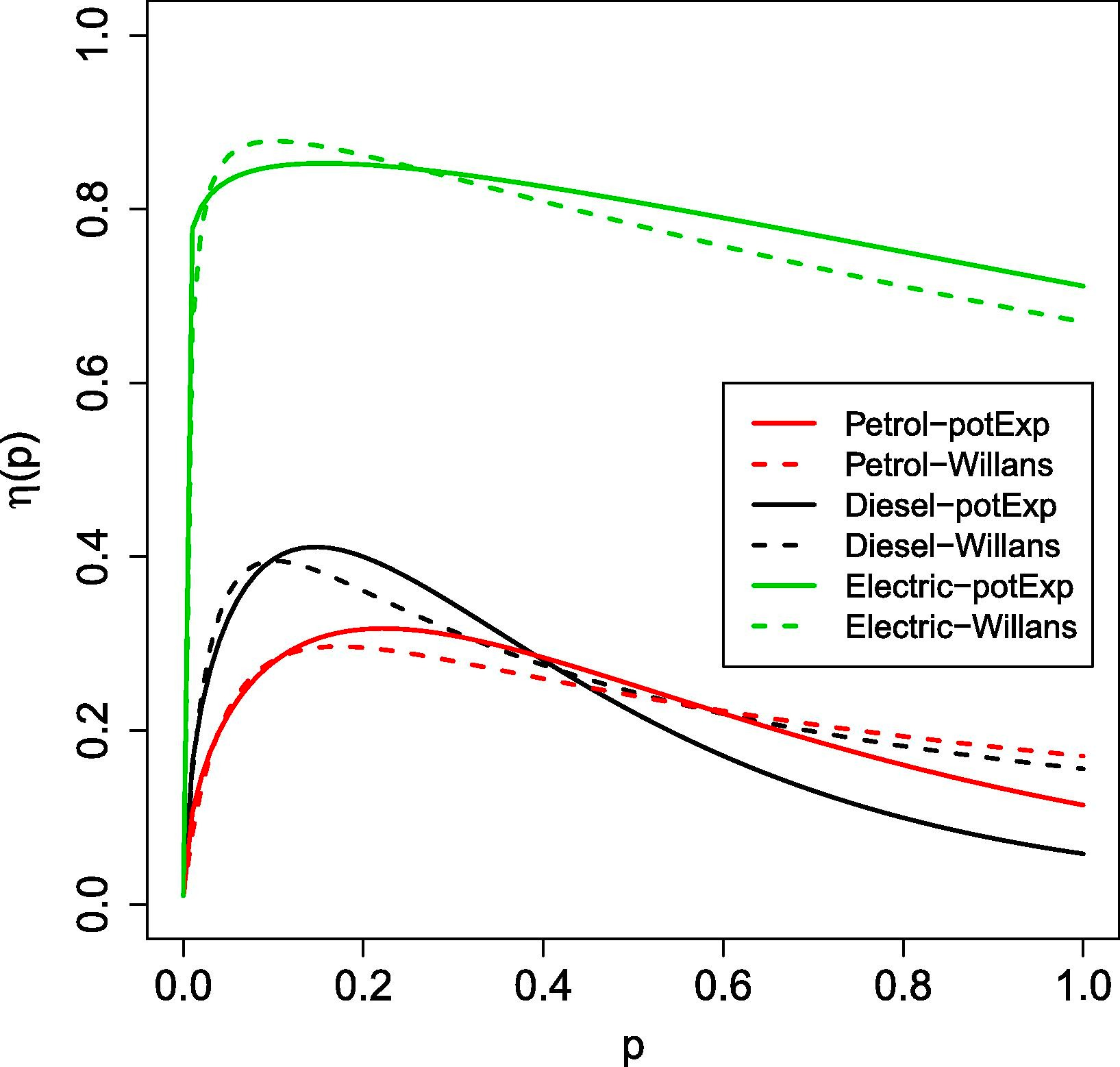
*Figure 8: Tank-to-wheel efficiency as a function of utilized power. Source: Hjelkrem et al. 2020 [Hjelkrem et al., 2020] *
For diesel and gasoline hybrid vehicles, the approach to estimating the engine and transmission efficiencies is similar, but a small electric motor allows for energy recuperation and reducing the engine size, which leads to higher efficiency levels. The amount of energy recuperated is determined by the driving cycle as well as the round-trip efficiency between the wheels and the engine and cannot be superior to the power output of the engine. Further on, the share of recuperated energy over the total negative motive energy (i.e., the braking or deceleration energy) is used as a discounting factor for brake wear particle emissions.
Electric energy storage
Battery electric vehicles can use different battery chemistry (Li-ion NMC, Li-ion LFP, Li-ion NCA and Li-LTO) depending on the manufacturer’s preference or the location of the battery supplier. Unless specified otherwise, all battery types are produced in China, as several sources, among which BloombergNEF [Henze, 2020], seem to indicate that more than 75% of the world’s cell capacity is manufactured there.
Accordingly, the electricity mix used for battery cells manufacture and drying, as well as the provision of heat are assumed to be representative of the country (i.e., the corresponding providers are selected from the LCI background database).
The battery-related parameters considered in carculator for 2020 are
shown in Table 6. For LFP batteries, “blade battery” or “cell-to-pack”
battery configurations are considered, as introduced by CATL [Xinhua, 2019] and BYD
[Mark, 2020], two major LFP battery suppliers in Asia. This greatly increases
the cell-to-pack ratio and the gravimetric energy density at the pack
level.
Overall, the gravimetric energy density values at the cell and system levels presented in Table 6 are considered conservative: some manufacturers perform significantly better than the average, and these values tend to change rapidly over time, as it is being the focus of much R&D. Hence, by 2050, the gravimetric energy density of NMC and NCA cells are expected to reach 0.5 kWh/kg, while that of LFP cells plateaus at 0.15 kWh/kg (but benefits from a high cell-to-pack ratio)..
Lithium Nickel Manganese Cobalt Oxide (LiNiMnCoO2) — NMC |
Lithium Iron Phosphate(LiFePO4) — LFP |
Lithium Nickel Cobalt Aluminum Oxide (LiNiCoAlO2) — NCA |
Source |
|
|---|---|---|---|---|
Cell energy density [kWh/kg] |
0.2 (0.5 in 2050) |
0.15 |
0.23 (0.5 in 2050) |
|
Cell-to-pack ratio |
0.6 (0.65 in 2050) |
0.8 (0.9 in 2050) |
0.5 (0.55 in 2050) |
|
Pack-level gravimetric energy density [kWh/kg] |
0.12 |
0.12 |
0.14 |
Calculated from the two rows above |
Share of cell mass in battery system [%] |
70 to 80% (depending on chemistry, see third row above) |
|||
Maximum state of charge [%] |
100% |
100% |
100% |
|
Minimum state of charge [%] |
20% |
20% |
20% |
|
Cycle life to reach 20% initial capacity loss (80%-20% SoC charge cycle) |
2’000 |
7’000+ |
1’000 |
|
Corrected cycle life |
3’000 |
7’000 |
1’500 |
Assumption |
Charge efficiency |
85% in 2020, 86% in 2050 |
[Brian and others, 2020, Brian and others, 2020] for passenger cars. |
||
Discharge efficiency |
88% in 2020, 89% in 2050 |
Note
The NMC battery cell used by default corresponds to a so-called NMC 6-2-2 chemistry: it exhibits three times the mass amount of Ni compared to Mn, and Co, while Mn and Co are present in equal amount. Development aims at reducing the content of Cobalt and increasing the Nickel share. A selection of other chemistry types can be chosen from.
On account that:
the battery cycle life values were obtained in the context of an experiment [Yuliya and others, 2020],
with loss of 20% of the initial capacity, the battery may still provide enough energy to complete the intended route, cycle life values for NMC and NCA battery chemistry are corrected by +50%.
Note
Important assumption: The environmental burden associated with the manufacture of spare batteries is entirely allocated to the vehicle use. The number of battery replacements is rounded up.
Table 7 gives an overview of the number of battery replacements assumed
for the different battery electric vehicles in carculator.
NMC |
LFP |
NCA |
|
|---|---|---|---|
Passenger car, electric, 2020 |
0 |
0 |
0 |
Passenger car, electric, 2050 |
0 |
0 |
0 |
Users are encouraged to test the sensitivity of end-results on the number of battery replacements.
The number of battery replacement is calculated as follows:
Where:
\(L_{veh}\) is the lifetime of the vehicle [km],
and \(L_{batt}\) is the lifetime of the battery [km].
Liquid and gaseous energy storage
The energy stored in the fuel (oxidation energy stored), the mass of the fuel tank for diesel, gasoline and compressed gas vehicles are calculated. Here are the formulas and units used:
- Calculate oxidation energy stored:
Oxidation energy stored (MWh) = fuel mass (kg) * LHV fuel (MJ/kg) / 3.6
- Calculate fuel tank mass for liquid fuels:
Fuel tank mass (kg) = oxidation energy stored (MWh) * fuel tank mass per energy (kg/MWh)
- Calculate fuel tank mass for compressed natural gas:
Fuel tank mass (kg) = oxidation energy stored (MWh) * CNG tank mass slope + CNG tank mass intercept
The set_energy_stored_properties function calculates the oxidation energy stored in the fuel, based on the fuel mass and the lower heating value (LHV) of the fuel. The fuel mass (in kilograms) is multiplied by the LHV fuel (in megajoules per kilogram), and the result is divided by 3.6 to convert the energy to megawatt-hours (MWh).
Next, the function calculates the mass of the fuel tank by multiplying the oxidation energy stored (in MWh) by the fuel tank mass per energy (in kilograms per MWh).
Lastly, if the powertrain is an ICEV-g, the function adjusts the fuel tank mass based on the oxidation energy stored and the coefficients for the CNG tank mass slope and intercept.
Note
The tank mass per unit of energy is different for liquid fuels (gasoline, diesel), and for gaseous fuels (compressed gas, hydrogen). Also, compressed gas tanks store at 200 bar, while hydrogen tanks store at 700 bar.
Fuel cell stack
All fuel cell electric vehicles use a proton exchange membrane (PEM)-based fuel cell system.
Table 8 lists the specifications of the fuel cell stack and system used
in carculator in 2020. The durability of the fuel cell stack,
expressed in hours, is used to determine the number of replacements
needed - the expected kilometric lifetime of the vehicle as well as the
average speed specified by the driving cycle gives the number of hours
of operation. The environmental burden associated with the manufacture
of spare fuel cell systems is entirely allocated to vehicle use as no
reuse channels seem to be implemented for fuel cell stacks at the
moment.
2020 |
2050 |
Source |
|
|---|---|---|---|
Power [kW] |
65 - 140 |
65 140 |
Calculated. |
Fuel cell stack efficiency [%] |
55-58% |
60% |
|
Fuel cell stack own consumption [% of kW output] |
15% |
12% |
|
Fuel cell system efficiency [%] |
45-50% |
53% |
|
Power density [W/cm2 cell] |
0.9 |
1 |
For passenger cars, [Simons and Bauer, 2015]. |
Specific mass [kg cell/W] |
0.51 |
||
Platinum loading [mg/cm2] |
0.13 |
||
Fuel cell stack durability [hours to reach 20% cell voltage degradation] |
4 000 |
5 625 |
|
Fuel cell stack lifetime replacements [unit] |
1 |
0 |
Calculated. |
The fuel cell system efficiency \(r_{fcsys}\) is calculated as:
Where:
\(r_{fcstack}\) is the fuel cell stack efficiency [%],
and \(r_{fcown}\) is the rate of auto consumption [%].
For reference, the rate of auto-consumption in 2020 for a fuel cell system is 15% (i.e., 15% of the power produced by the fuel cell system is consumed by it).
The fuel cell system power \(P_{fcsys}\) is calculated as:
Where:
\(P_{veh}\) is the vehicle engine power
and \(r_{fcshare}\) is the fuel cell system power relative to the vehicle engine power [%].
Finally, the fuel cell stack mass is calculated as:
Where:
\(P_{fcsys}\) is the fuel cell system power [kW],
\(A_{fc}\) is the fuel cell fuel cell power area density [kW/cm2],
and \(m_{fcstack}\) is the fuel cell stack mass [kg].
Note
Important remark: Although fuel cell electric vehicles have a small battery to enable the recuperation of braking energy, etc., we model it as a power battery, not a storage battery. For example, the Toyota Mirai is equipped with a 1.6 kWh nickel-based battery.
The battery power is calculated as:
Where:
\(P_{fcsys}\) is the fuel cell system power [kW],
and \(r_{fcshare}\) is the fuel cell system power share [%].
The number of fuel cell replacements is based on the average distance driven with a set of fuel cells given their lifetime expressed in hours of use. The number is replacement is rounded up as we assume no allocation of burden with a second life. It is hence is calculated as:
Where:
\(L_{veh}\) is the lifetime of the vehicle [km],
\(V_{avg}\) is the average speed of the driving cycle selected [km/h],
and \(L_{fc}\) is the fuel cell lifetime in hours [h].
Light-weighting
The automotive industry has been increasingly using light weighting materials to replace steel in engine blocks, chassis, wheels rims and powertrain components [Frontier, 2019]. However, vehicles light weighting has not led to an overall curb mass reduction for passenger cars and trucks, as additional safety equipment compensate for it. According to [Mock, 2017], passenger cars in the EU in 2016 were on average 10% heavier than in 2000.
The dataset used to represent the chassis of passenger cars (i.e., “glider, for passenger car”) does not reflect today’s use of light weighting materials, such as aluminium and advanced high strength steel (AHSS).
A report from the Steel Recycling Institute [Sebastian and Thimons, 2017] indicates that every kilogram of steel in a car glider can be substituted by 0.75 kilogram of AHSS or 0.68 kilogram of aluminium. Looking at the material composition of different car models three years apart, [Troy and others, 2017] show that steel is in fact increasingly replaced by a combination of both aluminium and AHSS. However, they also show that the use of AHSS is generally preferred to aluminium as its mass reduction-to-cost ratio is preferable.
Hence, it is considered that, for a given mass reduction to reach, two-third of the mass reduction comes from using AHSS, and one third comes from using aluminium. This means that one kilogram of mass reduction is achieved by replacing 3.57 kilogram of steel by:
1.76 kilogram of AHSS
0.8 kilogram of aluminium
Additionally, additional efforts is made to ensure that the final aluminium content in the chassis corresponds to what is actually found in current passenger car models, according to [Frontier, 2019].
While ecoinvent v.3.8 has a LCI dataset for the supply of aluminium, it is not the case for AHSS. However, an LCA report from the World Steel Institute [Association, 2015] indicates that AHSS has a similar carbon footprint than conventional primary low-alloyed steel from a basic oxygen furnace route (i.e., 2.3 kg CO2-eq./kg). We therefore use conventional steel to represent the use of AHSS.
The amount of light-weighting obtained from the use of light-weighting materials is:
\(\Delta m_{glider} = m_{glider} \times r_{lightweighting}\)
Where:
\(\Delta m_{steel}\) is the mass reduction of the glider [kg],
and \(r_{lightweighting}\) is the light-weighting ratio [%].
Sizing of onboard energy storage
Sizing of battery
The sizing of batteries for battery electric vehicles is conditioned by the battery mass, which is defined as an input parameter for each size class. The battery masses given for the different size classes are presented in Figure 9 using the battery chemistry NMC, and is based on representative battery storage capacities available today on the market - which are represented in relation to the curb mass. The data is collected from the vehicle’s registry of Touring Club Switzerland.
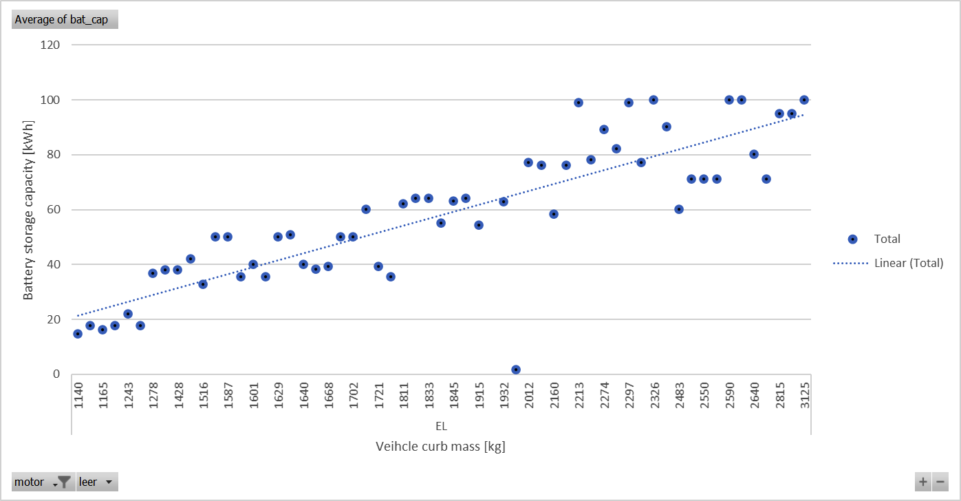
Figure 9: Energy storage capacity for current battery electric cars, shown in relation to curb mass. Red dots are the energy storage capacities used for Small, Medium and Large battery electric vehicles in ``carculator``
Seventy percent of the overall battery mass is assumed to be represented by the battery cells in the case of NMC and NCA batteries. Given the energy density of the battery cell considered, this yields the storage capacity of the battery. A typical depth of discharge of 80% is used to calculate the available storage capacity.
Unit |
Micro |
Small |
Medium |
Large |
Large SUV |
|
|---|---|---|---|---|---|---|
Storage capacity (reference) |
kWh |
14 |
35 |
45 |
70 |
80 |
Commercial models with similar energy storage capacity |
Microlino, Renault Twizzy |
VW e-Up!, BMW i3 |
Citroen e-C4, DS 3 E.Tense, Peugeot 2008, Peugeot 208, Opel Corsa-e, VW ID.3 |
Audi e-Tron, Tesla Model 3 |
Jaguar i-Pace |
|
Battery mass (system) |
Kilogram |
120 |
291 |
375 |
583 |
660 |
Battery cell mass |
% |
~70% |
||||
Battery cell mass |
Kilogram |
72 |
175 |
225 |
330 |
400 |
Balance of Plant mass |
Kilogram |
48 |
116 |
150 |
233 |
260 |
Energy density |
kWh/kg |
0.2 |
||||
Storage capacity |
kWh |
35 |
45 |
70 |
80 |
|
Depth of discharge |
% |
80% |
||||
Storage capacity (available) |
kWh |
14 |
28 |
36 |
56 |
65 |
Hence, the battery cell mass is calculated as:
Where:
\(m_{pack}\) is the mass of the pack,
and \(s_{cell}\) is the cell-to-pack ratio.
And the electricity stored in the battery is calculated as:
Where:
\(E_{battery}\) being battery capacity [kWh],
\(C_{cell}\) is the cell energy density [kg/kWh],
and \(m_{cell}\) is the cell mass [kg].
By deduction, the balance of plant mass is:
Where:
\(m_{battery}\) is the mass of the battery [kg],
and \(m_{cell}\) is the cell mass [kg].
Finally, the range autonomy is calculated as:
Where:
\(C_{battery}\) is the battery capacity [kWh],
\(r_{discharge}\) is the discharge depth [%],
and \(F_{ttw}\) is the tank-to-wheel energy consumption [kWh/km].
Similarly, plug-in hybrid vehicles are dimensioned to obtain an energy storage capacity of the battery that corresponds with the capacity of models available today. The sizing of the battery is similar to what is described above for battery electric vehicles. The energy storage capacity of the battery is particularly important for plugin hybrid vehicles, as it conditions the electric utility factor (the share of kilometers driven in battery-depleting mode) which calculation is described in the next section.
Unit |
Small |
Medium |
Large |
Large SUV |
|
|---|---|---|---|---|---|
Battery storage capacity (reference) |
kWh |
9 |
13 |
18 |
|
Commercial models with similar electric and fuel storage capacity |
Kia Niro, Kia Xceed |
Skoda Octavia, VW Golf, Cupra Leon |
Suzuki Across, VW Touareg |
||
Battery mass (system) |
Kilogram |
80 |
105 |
160 |
|
Battery cell mass |
% |
60% |
|||
Battery cell mass |
Kilogram |
48 |
63 |
96 |
|
Balance of Plant mass |
Kilogram |
32 |
42 |
64 |
|
Energy density |
kWh/kg |
0.2 |
|||
Battery storage capacity |
kWh |
9 |
13 |
19 |
|
Depth of discharge |
% |
80% |
|||
Battery storage capacity (available) |
kWh |
7.2 |
10.4 |
15.6 |
|
Fuel tank storage capacity |
L |
45 |
52 |
64 |
|
Note
carculator only considers NMC batteries for plugin hybrid vehicles.
Note
Important remark: Fuel cell vehicles are also equipped with a small battery. Its sizing is calculated differently. The battery capacity is calculated as:
Where:
\(E_{battery}\) being battery capacity [kWh],
\(P_{fcsys}\) is the fuel cell system power [kW],
\(r_{fcsys}\) is the fuel cell system power share [%],
and \(r_{discharge}\) is the discharge depth [%].
The battery mass is calculated as for battery electric vehicles, considering the cell energy density.
For example, for a small fuel cell vehicle with a fuel cell system power of 65 kW,
carculator will estimate a battery capacity of about 2 kWh.
Electric utility factor
Diesel and gasoline plugin hybrid vehicles are modeled as a composition of an ICE vehicle and a battery electric vehicle to the extent determined by the share of km driven in battery-depleting mode (also called “electric utility factor”). This electric utility factor is calculated based on a report from the ICCT [Patrick and others, 2020], which provides measured electricity utility factors for 6’000 PHEV private owners in Germany in relation to the vehicle range in battery-depleting mode.
A first step consists in determining the energy consumption of the PHEV in electric mode as well as its battery size, in order to know its range autonomy. When the range autonomy is known, the electric utility factor is interpolated based on the data presented in Table 11.
Range in battery-depleting mode [km] |
Observed electric utility factor [%] |
|---|---|
20 |
30 |
30 |
41 |
40 |
50 |
50 |
58 |
60 |
65 |
70 |
71 |
80 |
75 |
Once the electric utility factor \(U\) is known, it is used as a partitioning ratio to compose the vehicle between the PHEV in combustion mode, and the PHEV in electric mode, where:
Where:
\(F_{ttw_phev_e}\) is the tank-to-wheel energy consumption [kWh/km] of the electric PHEV,
\(F_{ttw_phev_c}\) is the tank-to-wheel energy consumption [kk/km] of the combustion PHEV,
\(m_{curb_phev_e}\) is the curb weight [kg] of the electric PHEV,
and \(m_{curb_phev_c}\) is the curb weight [kg] of the combustion PHEV.
Inventory modelling
Once the vehicles are modeled, the calculated parameters of each of them is passed to the inventory.py calculation module to derive inventories. When the inventories for the vehicle and the transport are calculated, they can be normalized by the kilometric lifetime (i.e., vehicle-kilometer) or by the kilometric multiplied by the passenger occupancy (i.e., passenger-kilometer).
Road demand
The demand for construction and maintenance of roads and road-related infrastructure is calculated on the following basis:
Road construction: 5.37e-7 meter-year per kg of vehicle mass per km.
Road maintenance: 1.29e-3 meter-year per km, regardless of vehicle mass.
The driving mass of the vehicle consists of the mass of the vehicle in running condition (including fuel) in addition to the mass of passengers and cargo, if any. Unless changed, the passenger mass is 75 kilograms, and the average occupancy is 1.6 persons per vehicle.
The demand rates used to calculate the amounts required for road construction and maintenance (based on vehicle mass per km and per km, respectively) are taken from [Spielmann and Scholz, 2005].
Because roads are maintained by removing surface layers older than those that are actually discarded, road infrastructure disposal is modeled in ecoinvent as a renewal rate over the year in the road construction dataset.
Vehicle maintenance
The modelling of the maintenance life.cycle phase is simple. It is based on the ecoinvent’s dataset for the maintenance of a 1,250 kg gasoline-run VW Golf IV. carculator simply normalize the input requirements per kg of vehicle to maintain, and multiply them by the vehicle mass.
Note
Important remark: This approach often leads to electric vehicles having a higher maintenance-related burden, because of their higher mass – which may not be the case in reality. It is hence an aspect to be improved in the future.
Fuel properties
For all vehicles with an internal combustion engine, carbon dioxide (CO2) and sulfur dioxide (SO2) emissions are calculated based on the fuel consumption of the vehicle and the carbon and sulfur concentration of the fuel observed in Switzerland and Europe. Sulfur concentration values are sourced from HBEFA 4.1 [Benedikt and others, 2019]. Lower heating values and CO2 emission factors for fuels are sourced from p.86 and p.103 of [for the Environment, 2021]. The fuel properties shown in Table 12 are used for fuels purchased in Switzerland.
Volumetric mass density [kg/l] |
Lower heating value [MJ/kg] |
CO2 emission factor [kg CO2/kg] |
SO2 emission factor [kg SO2/kg] |
|
|---|---|---|---|---|
Gasoline |
0.75 |
42.6 |
3.14 |
1.6e-5 |
Bioethanol |
0.75 |
26.5 |
1.96 |
1.6e-5 |
Synthetic gasoline |
0.75 |
43 |
3.14 |
0 |
Diesel |
0.85 |
43 |
3.15 |
8.85e-4 |
Biodiesel |
0.85 |
38 |
2.79 |
8.85e-4 |
Synthetic diesel |
0.85 |
43 |
3.15 |
0 |
Natural gas |
47.5 |
2.68 |
||
Bio-methane |
47.5 |
2.68 |
||
Synthetic methane |
47.5 |
2.68 |
Because large variations are observed in terms of sulfur concentration in biofuels, similar values than that of conventional fuels are used.
Exhaust emissions
Emissions of regulated and non-regulated substances during driving are approximated using emission factors from HBEFA 4.1 [Benedikt and others, 2019]. Emission factors are typically given in gram per km. Emission factors representing free flowing driving conditions and urban and rural traffic situations are used. Additionally, cold start emissions as well as running, evaporation and diurnal losses are accounted for, also sourced from HBEFA 4.1 [Benedikt and others, 2019].
For vehicles with an internal combustion engine, the sulfur concentration values in the fuel can slightly differ across regions - although this remains rather limited within Europe. The values provided by HBEFA 4.1 are used for Switzerland, France, Germany, Austria and Sweden. For other countries, values from [Miller and Jin, 2019] are used.
Sulfur [ppm/fuel wt.] |
Switzerland |
Europe |
|---|---|---|
Gasoline |
8 |
8 |
Diesel |
10 |
8 |
The amount of sulfur dioxide released by the vehicle over one km [kg/km] is calculated as:
Where:
\(r_{S}\) is the sulfur content per kg of fuel [kg SO2/kg fuel],
\(F_{fuel}\) is the fuel consumption of the vehicle [kg/km],
and \(64/32\) is the ratio between the molar mass of SO2 and the molar mass of O2.
Country-specific fuel blends are sourced from the IEA’s Extended World Energy Balances database [(IEA), 2021]. By default, the biofuel used is assumed to be produced from biomass residues (i.e., second-generation fuel): fermentation of crop residues for bioethanol, esterification of used vegetable oil for biodiesel and anaerobic digestion of sewage sludge for bio-methane.
Biofuel share [% wt.] |
Switzerland |
Europe |
|---|---|---|
Gasoline blend |
1.2 |
4 |
Diesel blend |
4.8 |
6 |
Compressed gas blend |
22 |
9 |
A number of fuel-related emissions other than CO2 and SO2 are considered, using the HBEFA 4.1 database [Benedikt and others, 2019].
Six sources of emissions are considered:
Exhaust emissions: emissions from the combustion of fuel during operation. Their concentration relates to the fuel consumption and the emission standard of the vehicle.
Cold start emissions: emissions when starting the engine. The factor is given in grams per engine start. 2.3 engine starts per day are considered [for the Environment, 2021] and an annual mileage of 12’000 km.
Diurnal emissions: evaporation of the fuel due to a temperature increase of the vehicle. The factor is given in grams per day. Emissions are distributed evenly along the driving cycle, based on an annual mileage of 12’000 km per year.
Hot soak emissions: evaporative emissions occurring after the vehicle has been used. The factor is given in grams per trip. The emission is added at the end of the driving cycle.
In addition, running loss emissions: emissions related to the evaporation of fuel (i.e., not combusted) during operation. The factor is given in grams per km. Emissions are distributed evenly along the driving cycle.
Other non-exhaust emissions: brake, tire road wear and re-suspended road dust emissions, as well as emissions of refrigerant.
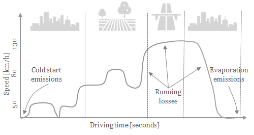
Figure 10: Representation of the different sources of emission other than exhaust emissions
For exhaust emissions, factors based on the fuel consumption are derived by comparing emission data points for different traffic situations (i.e., grams emitted per vehicle-km) for in a free flowing driving situation, with the fuel consumption corresponding to each data point (i.e., MJ of fuel consumed per km), as illustrated in Figure 11 for a diesel-powered engine. The aim is to obtain emission factors expressed in grams of substance emitted per MJ of fuel consumed, to be able to model emissions of passenger cars of different sizes and fuel efficiency and for different driving cycles.
Hence, the emission of substance i at second s of the driving cycle is calculated as follows:
Where:
\(E(i,s)\) is the emission of substance i at second s of the driving cycle,
\(F_ttw(s)\) is the fuel consumption of the vehicle at second s,
and \(X(i, e)\) is the emission factor of substance i in the given driving conditions.
To that, we add the following terms:
Cold start emissions on the first second of the driving cycle
Evaporation emissions: on the last second of the driving cycle
Diurnal and running losses: distributed evenly over the driving cycle
Note
Important remark: the degradation of anti-pollution systems for
diesel and gasoline cars (i.e., catalytic converters) is accounted for
as indicated by HBEFA, by applying a degradation factor on the emission
factors for CO, HC and NOx for gasoline cars, as well as on CO
and NOx for diesel cars. These factors are shown in Table 15
for passenger cars with a mileage of 200’000 km, which is the default
lifetime value in carculator. The degradation factor corresponding to
half of the vehicle kilometric lifetime is used, to obtain a
lifetime-weighted average degradation factor.
Degradation factor at 200 000 km |
Gasoline passenger cars |
Diesel passenger cars |
|||
|---|---|---|---|---|---|
CO |
HC |
NOx |
CO |
NOx |
|
EURO-1 |
1.9 |
1.59 |
2.5 |
||
EURO-2 |
1.6 |
1.59 |
2.3 |
1.25 |
|
EURO-3 |
1.75 |
1.02 |
2.9 |
1.2 |
|
EURO-4 |
1.9 |
1.02 |
2 |
1.3 |
1.06 |
EURO-5 |
2 |
2.5 |
1.3 |
1.03 |
|
EURO-6 |
1.3 |
1.3 |
1.4 |
1.15 |
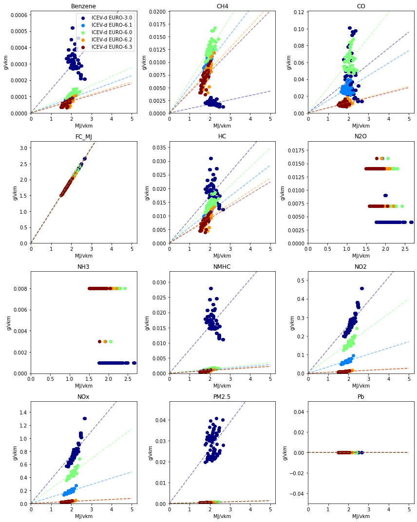
Figure 11: Relation between emission factor and fuel consumption for a diesel-powered passenger car. Dots represent HBEFA 4.1 emission factors for different traffic situation for a diesel engine, for different emission standards
However, as Figure 11 shows, the relation between amounts emitted and fuel consumption is not always obvious and using a linear relation between amounts emitted and fuel consumption can potentially be incorrect. In addition, emissions of ammonia (NH3) and Nitrous oxides (N2O) seem to be related to the emission standard (e.g., use of urea solution) and engine temperature rather than the fuel consumption.
To confirm that such approach does not yield kilometric emissions too
different from the emission factors per vehicle-kilometer proposed by
HBEFA 4.1, Figure 12 compares the emissions obtained by carculator
using the WLTC driving cycle over 1 vehicle-km (red dots) with the
distribution of the emission factors for different traffic situations
(green box-and-whiskers) as well as the traffic situation-weighted
average emission factor (yellow dots) given by HBEFA 4.1 for different
emission standards for a medium diesel-powered passenger car.
There is some variation across traffic situations, but the emissions obtained remain, for most substances, within the 50% of the distributed HBEFA values across traffic situations. Also, the distance between the modeled emission and the traffic-situation-weighted average is reasonable.
Note
Important remark: NOx emissions for emission standards
EURO-4 and 5 tend to be under-estimated compared to HBEFA’s values. It
is also important to highlight that, in some traffic situations, HBEFA’s
values show that emissions of CO, HC, NMHC and PMs for vehicles with
early emission standards can be much higher that what is assumed in
carculator. There is overall a good agreement between traffic
situation-weighted average emission factors and those used in
carculator.
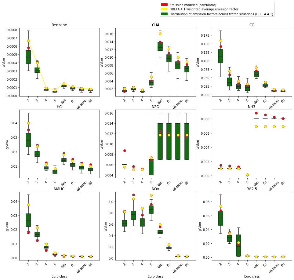
Figure 12 Validation of the exhaust emissions model with the emission factors provided by HBEFA 4.1 for a medium size diesel-powered passenger car. Box-and-whiskers: distribution of HBEFA’s emission factors for different traffic situations (box: 50% of the distribution, whiskers: 90% of the distribution). Yellow dots: traffic situation-weighted average emission factors. Red dots: modeled emissions calculated by ``carculator`` with the WLTC cycle, using the relation between fuel consumption and amounts emitted
NMHC speciation
After NMHC emissions are quantified, EEA/EMEP’s 2019 Air Pollutant Emission Inventory Guidebook provides factors to further specify some of them into the substances listed in Table 16.
All gasoline vehicles
|
All diesel vehicles
|
|
|---|---|---|
Ethane |
3.2 |
0.33 |
Propane |
0.7 |
0.11 |
Butane |
5.2 |
0.11 |
Pentane |
2.2 |
0.04 |
Hexane |
1.6 |
0 |
Cyclohexane |
1.1 |
0.65 |
Heptane |
0.7 |
0.2 |
Ethene |
7.3 |
10.97 |
Propene |
3.8 |
3.6 |
1-Pentene |
0.1 |
0 |
Toluene |
11 |
0.69 |
m-Xylene |
5.4 |
0.61 |
o-Xylene |
2.3 |
0.27 |
Formaldehyde |
1.7 |
12 |
Acetaldehyde |
0.8 |
6.47 |
Benzaldehyde |
0.2 |
0.86 |
Acetone |
0.6 |
2.94 |
Methyl ethyl ketone |
0.1 |
1.2 |
Acrolein |
0.2 |
3.58 |
Styrene |
1 |
0.37 |
NMVOC, unspecified |
50.8 |
55 |
Non-exhaust emissions
A number of emission sources besides exhaust emissions are considered. They are described in the following sub-sections.
Engine wear emissions
Metals and other substances are emitted during the combustion of fuel because of engine wear. These emissions are scaled based on the fuel consumption, using the emission factors listed in Table 17, sourced from [Agency, 2019].
All gasoline vehicles
|
All diesel vehicles
|
|
|---|---|---|
PAH |
8.19E-10 |
1.32E-09 |
Arsenic |
7.06E-12 |
2.33E-12 |
Selenium |
4.71E-12 |
2.33E-12 |
Zinc |
5.08E-08 |
4.05E-08 |
Copper |
9.88E-10 |
4.93E-10 |
Nickel |
3.06E-10 |
2.05E-10 |
Chromium |
3.76E-10 |
6.98E-10 |
Chromium VI |
7.53E-13 |
1.40E-12 |
Mercury |
2.05E-10 |
1.23E-10 |
Cadmium |
2.54E-10 |
2.02E-10 |
Abrasion emissions
We distinguish four types of abrasion emissions, besides engine wear emissions:
brake wear emissions: from the wearing out of brake drums, discs and pads
tires wear emissions: from the wearing out of rubber tires on the asphalt
road wear emissions: from the wearing out of the road pavement
and re-suspended road dust: dust on the road surface that is re-suspended as a result of passing traffic, “due either to shear forces at the tire/road surface interface, or air turbulence in the wake of a moving vehicle” [Beddows and Harrison, 2021].
[Beddows and Harrison, 2021] provides an approach for estimating the mass and extent of these abrasion emissions. They propose to disaggregate the abrasion emission factors presented in the EMEP’s 2019 Emission inventory guidebook [Agency, 2019] for two-wheelers, passenger cars, buses and heavy good vehicles, to re-quantify them as a function of vehicle mass, but also traffic situations (urban, rural and motorway). Additionally, they present an approach to calculate re-suspended road dust according to the method presented in [EPA, 2011] - such factors are not present in the EMEP’s 2019 Emission inventory guidebook - using representative values for dust load on European roads.
The equation to calculate brake, tire, road and re-suspended road dust emissions is the following:
With:
\(EF\) being the emission factor, in mg per vehicle-kilometer
\(W\) being the vehicle mass, in tons
\(b\) and \(c\) being regression coefficients, whose values are presented in Table 18.
Tire wear |
Brake wear |
Road wear |
Re-suspended road dust |
|||||||||||||
|---|---|---|---|---|---|---|---|---|---|---|---|---|---|---|---|---|
Urban |
Rural |
Motorway |
Urban |
Rural |
Motorway |
|||||||||||
b |
c |
b |
c |
b |
c |
b |
c |
b |
c |
b |
c |
b |
c |
b |
c |
|
PM 10 |
5.8 |
2.3 |
4.5 |
2.3 |
3.8 |
2.3 |
4.2 |
1.9 |
1.8 |
1.5 |
0.4 |
1.3 |
2.8 |
1.5 |
2 |
1.1 |
PM 2.5 |
8.2 |
2.3 |
6.4 |
2.3 |
5.5 |
2.3 |
11 |
1.9 |
4.5 |
1.5 |
1 |
1.3 |
5.1 |
1.5 |
8.2 |
1.1 |
The respective amounts of brake and tire wear emissions in urban, rural and motorway driving conditions are weighted, to represent the driving cycle used. The weight coefficients sum to 1 and the coefficients considered are presented in Table 19. They have been calculated by analyzing the speed profile of each driving cycle, with the exception of two-wheelers, for which no driving cycle is used (i.e., the energy consumption is from reported values) and where simple assumptions are made in that regard instead.
Driving cycle |
Urban |
Rural |
Motorway |
|
|---|---|---|---|---|
Passenger car |
WLTP |
0.33 |
0.24 |
0.43 |
Finally, for electric and (plugin) hybrid vehicles, the amount of brake wear emissions is reduced. This reduction is calculated as the ratio between the sum of energy recuperated by the regenerative braking system and the sum of negative resistance along the driving cycle. The logic is that the amount of negative resistance that could not be met by the regenerative braking system needs to be met with mechanical brakes. This is illustrated in Figure 13, where the distance between the recuperated energy and the total negative motive energy corresponds to the amount of energy that needs to be provided by mechanical brakes. Table 20 lists such reduction actors for the different powertrains.
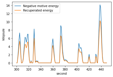
Figure 13: Negative motive energy and recuperated energy between second 300 and 450 of the WLTC driving cycle
Driving cycle |
Reduction factor for hybrid vehicles |
Reduction factor for plugin hybrid vehicles |
Reduction factor for battery and fuel cell electric vehicles |
|
|---|---|---|---|---|
Passenger car |
WLTP |
-72% |
-73% |
-76% |
The sum of PM 2.5 and PM 10 emissions is used as the input for the ecoinvent v.3.x LCI datasets indicated in Table 21.
Tire wear |
Brake wear |
Road wear |
R e-suspended road dust |
|
|---|---|---|---|---|
Passenger car |
Tire wear emissions, passenger car |
Brake wear emissions, passenger car |
Road wear emissions, passenger car |
Finally, we assume that the composition of the re-suspended road dust is evenly distributed between brake, road and tire wear particles.
Figure 14 shows the calculated abrasion emissions for passenger cars in mg per vehicle-kilometer, following the approach presented above.
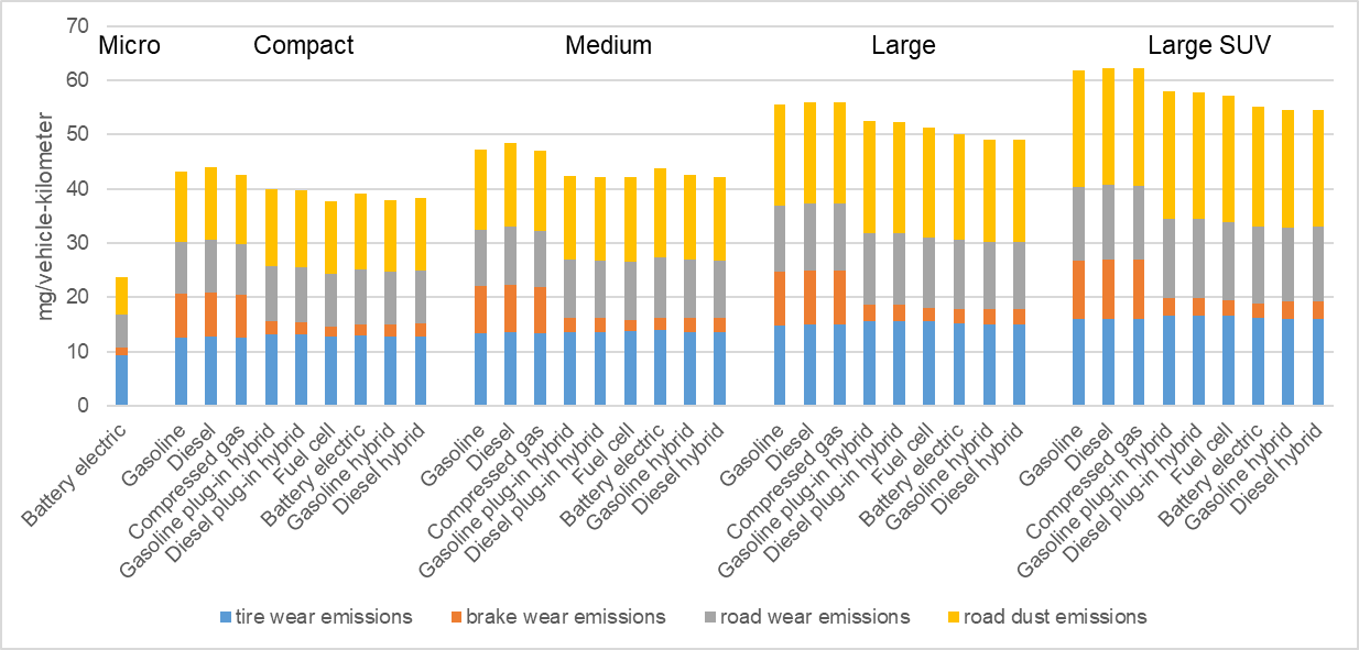
Figure 14: Total particulate matter emissions (<2.5 µm and 2.5-10 µm) in mg per vehicle-kilometer for passenger cars
Re-suspended road dust emissions are assumed to be evenly composed of brake wear (33.3%), tire wear (33.3%) and road wear (33.3%) particles.
Refrigerant emissions
The use of refrigerant for onboard air conditioning systems is considered for passenger cars until 2021. The supply of refrigerant gas R134a is accounted for. Similarly, the leakage of the refrigerant is also considered. For this, the calculations from [P. and others, 2016] are used. Such emission is included in the transportation dataset of the corresponding vehicle. The overall supply of refrigerant amounts to the initial charge plus the amount leaked throughout the lifetime of the vehicle, both listed in Table 22 This is an important aspect, as the refrigerant gas R134a has a Global Warming potential of 2’400 kg CO2-eq./kg released in the atmosphere.
Passenger cars (except Micro) |
|
|---|---|
Initial charge [kg per vehicle lifetime] |
0.55 |
Lifetime loss [kg per vehicle lifetime] |
0.75 |
Note
Important assumption: It is assumed that electric and plug-in electric vehicles also use a compressor-like belt-driven air conditioning system, relying on the refrigerant gas R134a. In practice, an increasing, but still minor, share of electric vehicles now use a (reversible) heat pump to provide cooling.
Note
Important remark: Micro cars do not have an air conditioning system. Hence, no supply or leakage of refrigerant is considered for those.
Note
Important remark: After 2021, R134a is no longer used.
Noise emissions
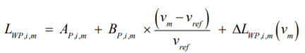
Noise emissions along the driving cycle of the vehicle are quantified using the method developed within the CNOSSOS project [Kephalopoulos and others, 2012], which are expressed in joules, for each of the 8 octaves. Rolling and propulsion noise emissions are quantified separately.
The sound power level of rolling noise is calculated using:
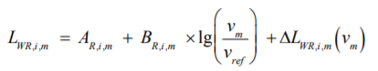
With:
\(v_m\) being the instant speed given by the driving cycle, in km/h
\(v_{ref}\) being the reference speed of 70 km/h
and \(A_{P,i,m}\) and \(B_{P,i,m}\) are unit-less and given in Table 23.
The propulsion noise level is calculated using:
With:
\(v_m\) being the instant speed given by the driving cycle, in km/h
\(v_{ref}\) being the reference speed of 70 km/h
and \(A_{P,i,m}\) and \(B_{P,i,m}\) are unit-less and given in Table 23.
Octave band center frequency (Hz) |
\(A_R\) |
\(B_R\) |
\(A_P\) |
\(B_P\) |
|---|---|---|---|---|
63 |
84 |
30 |
101 |
-1.9 |
125 |
88.7 |
35.8 |
96.5 |
4.7 |
250 |
91.5 |
32.6 |
98.8 |
6.4 |
500 |
96.7 |
23.8 |
96.8 |
6.5 |
1000 |
97.4 |
30.1 |
98.6 |
6.5 |
2000 |
90.9 |
36.2 |
95.2 |
6.5 |
4000 |
83.8 |
38.3 |
88.8 |
6.5 |
8000 |
80.5 |
40.1 |
82.7 |
6.5 |
A correction factor for battery electric and fuel cell electric vehicles is applied, and is sourced from [Pallas and others, 2016]. Also, electric vehicles are added a warning signal of 56 dB at speed levels below 20 km/h. Finally, hybrid vehicles are assumed to use an electric engine up to a speed level of 30 km/h, beyond which the combustion engine is used.
The total noise level (in A-weighted decibels) is calculated using the following equation:
The total sound power level is converted into Watts (or joules per second), using the following equation:
The total sound power, for each second of the driving cycle, is then distributed between the urban, suburban and rural inventory emission compartments.
Figure 15 illustrates a comparison of noise levels between an ICEV and BEV as calculated by the tool, over the driving cycle WLTC. In this figure, the noise levels at different frequency ranges have been summed together to obtain a total noise level (in dB), and converted to dB(A) using the A-weighting correction factor, to better represent the “loudness” or discomfort to the human ear. Typically, propulsion noise emissions dominate in urban environments (which corresponds to the Road demand section of the driving cycle), thereby justifying the use of electric vehicles in that regard. This is represented by the difference between the ICEV and BEV lines in the Road demand section of the driving cycle in Figure 15. The difference in noise level between the two powertrains diminishes at higher speed levels (see Fuel properties, Exhaust emissions and Non-exhaust emissions) as rolling noise emissions dominate above a speed level of approximately 50 km/h. This can be seen in Figure 16, which sums up the sound energy produced, in joules, over the course of the driving cycle.
The study from [Stefano and others, 2019] provides compartment-specific noise emission characterization factors against midpoint and endpoint indicators - expressed in Person-Pascal-second and Disability-Adjusted Life Year, respectively.
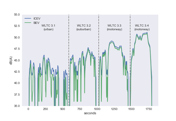
Figure 15: Noise emission level comparison between ICEV and BEV, based on the driving cycle WLTC
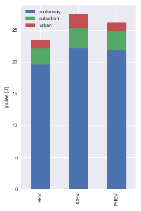
Figure 16: Summed sound energy comparison between ICEV, BEV and PHEV, over the duration of the WLTC driving cycle
Electricity mix calculation
Electricity supply mix are calculated based on the weighting from the
distribution the lifetime kilometers of the vehicles over the years of
use. For example, should a BEV enter the fleet in Poland in 2020, most
LCA models of passenger vehicles would use the electricity mix for
Poland corresponding to that year, which corresponds to the row of the
year 2020 in Table 24, based on ENTSO-E’s TYNDP 2020 projections
(National Trends scenario) [ENTSO-E, 2020]. carculator calculates instead the
average electricity mix obtained from distributing the annual kilometers
driven along the vehicle lifetime, assuming an equal number of
kilometers is driven each year. Therefore, with a lifetime of 200,000 km
and an annual mileage of 12,000 kilometers, the projected electricity
mixes to consider between 2020 and 2035 for Poland are shown in Table 24.
Using the kilometer-distributed average of the projected mixes
between 2020 and 2035 results in the electricity mix presented in the
last row of Table 24. The difference in terms of technology contribution
and unitary GHG-intensity between the electricity mix of 2020 and the
electricity mix based on the annual kilometer distribution is
significant (-23%). The merit of this approach ultimately depends on
whether the projections will be realized or not.
It is also important to remember that the unitary GHG emissions of each electricity-producing technology changes over time, as the background database ecoinvent has been transformed by premise [Sacchi and others, 2022]: for example, photovoltaic panels become more efficient, as well as some of the combustion-based technologies (e.g., natural gas). For more information about the transformation performed on the background life cycle database, refer to [Sacchi and others, 2022].
year |
Biomass |
Coal |
Gas |
Gas CCGT |
Gas CHP |
Hydro |
Hydro, reservoir |
Lignite |
Nuclear |
Oil |
Solar |
Waste |
Wind |
Wind, offshore |
g CO2-eq./kWh |
|---|---|---|---|---|---|---|---|---|---|---|---|---|---|---|---|
2020 |
3% |
46% |
2% |
3% |
0% |
3% |
1% |
29% |
3% |
0% |
0% |
0% |
9% |
0% |
863 |
2021 |
2% |
43% |
2% |
4% |
1% |
3% |
1% |
29% |
2% |
0% |
1% |
3% |
9% |
0% |
841 |
2022 |
2% |
41% |
1% |
5% |
1% |
3% |
1% |
28% |
2% |
0% |
2% |
5% |
9% |
0% |
807 |
2023 |
1% |
38% |
1% |
5% |
2% |
2% |
1% |
28% |
1% |
0% |
3% |
8% |
10% |
0% |
781 |
2024 |
1% |
36% |
0% |
6% |
2% |
2% |
0% |
27% |
1% |
0% |
3% |
11% |
10% |
0% |
745 |
2025 |
0% |
33% |
0% |
7% |
3% |
2% |
0% |
27% |
0% |
0% |
4% |
13% |
10% |
0% |
724 |
2026 |
0% |
31% |
0% |
8% |
3% |
2% |
0% |
25% |
0% |
0% |
5% |
13% |
11% |
2% |
684 |
2027 |
0% |
28% |
0% |
9% |
4% |
2% |
0% |
24% |
0% |
0% |
6% |
12% |
12% |
3% |
652 |
2028 |
0% |
25% |
0% |
9% |
5% |
2% |
0% |
23% |
0% |
0% |
6% |
12% |
13% |
5% |
614 |
2029 |
0% |
23% |
0% |
10% |
6% |
2% |
0% |
21% |
0% |
0% |
7% |
11% |
14% |
6% |
580 |
2030 |
0% |
20% |
0% |
11% |
6% |
2% |
0% |
20% |
0% |
0% |
8% |
10% |
15% |
8% |
542 |
2031 |
0% |
19% |
0% |
11% |
7% |
2% |
0% |
18% |
1% |
0% |
9% |
10% |
16% |
8% |
514 |
2032 |
0% |
17% |
0% |
10% |
8% |
2% |
0% |
16% |
3% |
0% |
9% |
9% |
17% |
9% |
470 |
2033 |
0% |
16% |
0% |
10% |
8% |
2% |
0% |
14% |
4% |
0% |
10% |
8% |
17% |
10% |
437 |
2034 |
0% |
15% |
0% |
10% |
9% |
2% |
0% |
12% |
5% |
0% |
10% |
8% |
18% |
11% |
408 |
2035 |
0% |
13% |
0% |
9% |
10% |
2% |
0% |
11% |
7% |
0% |
11% |
7% |
19% |
12% |
377 |
Mix |
0% |
26% |
0% |
7% |
5% |
2% |
0% |
21% |
2% |
0% |
6% |
8% |
13% |
5% |
668 |
Life cycle inventory modelling
Once the vehicles are specified, the material and energy inputs and emission outputs occuring throughout the different phases of their life-cycle are linked to life-cycle assessment datasets. Those are either sourced from the literature, or from the life-cycle assessment database ecoinvent.
The table below shows the correspondence between vehicle components and the life-cycle assessment datasets used.
Component Concerns Dataset name Source Glider All market for glider, passenger car ecoinvent Lightweighting material All
Inventories for fuel pathways
A number of inventories for fuel production and supply are used by
carculator. They represent an update in comparison to the inventories
used in the passenger vehicles model initially published by [Brian and others, 2020].
The fuel pathways presented in Table 25 are from the literature
and not present as generic ecoinvent datasets.
Author(s) |
Fuel type |
Description |
|---|---|---|
Bioethanol from forest residues |
Biofuels made from biomass residues (e.g., wheat straw, corn starch) or energy crops (e.g., sugarbeet). For energy crops biofuels, indirect land use change is included. |
|
Bioethanol from wheat straw |
||
Bioethanol from corn starch |
||
Bioethanol from sugarbeet |
||
e-Gasoline (Methanol-to-Gasoline) |
Gasoline produced from methanol, via a Methanol-to-Gasoline process. The carbon monoxide is provided by a reverse water gas shift process, feeding on carbon dioxide from direct air capture. In carculator, one can choose the nature of the heat needed for the methanol distillation as well as for regenerating the DAC sorbent: natural gas, waste heat, biomass heat, or market heat (i.e., a mix of natural gas and fuel oil). |
|
Biodiesel from micro-algae |
2nd and 3rd generation biofuels made from biomass residues or algae. |
|
Biodiesel from used cooking oil |
||
e-Diesel (Fischer-Tropsch) |
Diesel produced from
“blue crude” via a
Fischer-Tropsch process.
The H2 is
produced via
electrolysis, while the
CO2 comes from
direct air capture. Note
that in |
|
Biomethane from sewage sludge |
Methane produced from the anaerobic digestion of sewage sludge. The biogas is upgraded to biomethane (the CO2 is separated and vented out) to a vehicle grade quality. |
|
Synthetic methane |
Methane produced via an electrochemical methanation process, with H2 from electrolysis and CO2 from direct air capture. |
|
Hydrogen from electrolysis |
The electricity requirement to operate the electrolyzer changes over time: from 58 kWh per kg of H2 in 2010, down to 44 kWh in 2050, according to [Christian and others, 2021]. |
|
Hydrogen from Steam Methane Reforming |
Available for natural gas and biomethane, with and without Carbon Capture and Storage (CCS). |
|
Hydrogen from woody biomass gasification |
Available with and without Carbon Capture and Storage (CCS). |
Inventories for energy storage components
The source for the inventories used to model energy storage components are listed in Table 26.
Author(s) |
Energy storage type |
Description |
|---|---|---|
NMC-111/622/811 battery |
Originally from [Qiang and others, 2019], then updated and integrated in ecoinvent v.3.8 (with some errors), corrected and integrated in the library. Additionally, these inventories relied exclusively on synthetic graphite. This is has too been modified: the anode production relies on a 50:50 mix of natural and synthetic graphite, as it seems to be the current norm in the industry [James and Dan, 2019]. Inventories for natural graphite are from [Engels et al., 2022]. |
|
NCA battery |
||
LFP battery |
||
Type IV hydrogen tank, default |
Carbon fiber being one of
the main components of
Type IV storage tanks,
new inventories for
carbon fiber
manufacturing have been
integrated to
|
|
Type IV hydrogen tank, LDPE liner |
||
Type IV hydrogen tank, aluminium liner |
Life cycle impact assessment
To build the inventory of every vehicle, carculator populates a
three-dimensional array A (i.e., a tensor) such as:
The second and third dimensions (i.e., M and N) have the same
length. They correspond to product and natural flow exchanges between
supplying activities (i.e., M) and receiving activities (i.e., N).
The first dimension (i.e., L) stores model iterations. Its length
depends on whether the analysis is static or if an uncertainty analysis
is performed (e.g., Monte Carlo).
Given a final demand vector f (e.g., 1 kilometer driven with a
specific vehicle, represented by a vector filled with zeroes and the
value 1 at the position corresponding to the index j of the driving
activity in dimension M) of length equal to that of the second dimension
of A (i.e., M), carculator calculates the scaling factor s so
that:
Finally, the scaling factor s is multiplied with a characterization
matrix B. This matrix contains midpoint characterization factors for a
number of impact assessment methods (as rows) for every activity in A
(as columns).
As described earlier, the tool chooses between several
characterization matrices B, which contain pre-calculated values for
activities for a given year, depending on the year of production of the
vehicle as well as the REMIND climate scenario considered (i.e.,
“SSP2-Baseline”, “SSP2-PkBudg1150” or “SSP2-PkBudg500”). Midpoint and
endpoint (i.e., human health, ecosystem impacts and resources use)
indicators include those of the ReCiPe 2008 v.1.13 impact assessment
method, as well as those of EF 3.1. Additionally, it is possible to
export the inventories in a format compatible with the LCA framework
Brightway2 or SimaPro,
thereby allowing the characterization of the results against a larger number of impact assessment methods.
Presentation of results
Life-cycle impacts are presented across the following categories/life-cycle phases:
direct - exhaust
direct - non-exhaust
energy chain
powertrain
glider
energy storage
maintenance
end-of-life
road
A comprehensive presentation of life-cycle assessment (LCA) results for passenger cars should offer insights into various aspects that contribute to the overall environmental impact. Each category or life-cycle phase addresses a different set of environmental impacts, and assessing them individually helps to paint a complete picture. Below is an extended description of each category or life-cycle phase:
Direct - Exhaust
Description: This category evaluates the environmental impacts associated with the direct emissions from the vehicle’s exhaust system, including greenhouse gases (GHGs), particulate matter (PM), and volatile organic compounds (VOCs).
Substances measured:
Carbon dioxide (CO2)
Nitrogen oxides (NOx)
Particulate matter (PM)
Hydrocarbons
VOCs
Note that not all substance contribute to all impact categories. For example, NOx and VOCs contribute to the formation of ozone, but not to climate change.
Direct - Non-Exhaust
Description: This section focuses on emissions and impacts not related to the exhaust system, such as brake and tire wear, as well as emissions from air conditioning.
Parameters measured:
PM from brake, tire, road and engine wear, as well as re-suspended dust
Refrigerant losses (e.g., R143a) from air conditioning
Energy Chain
Description: Assesses the environmental impacts associated with the production, transportation, and distribution of the energy source used in the vehicle, be it gasoline, electricity, hydrogen, or any other.
Parameters Measured:
Energy source extraction impacts
Transportation emissions
Energy generation, transmission and distribution emissions
Powertrain
Description: This part examines the environmental burden from the manufacturing, operation, and disposal of the vehicle’s engine and transmission systems.
Parameters Measured:
Raw material extraction
Manufacturing emissions
Operational efficiency
Glider
Description: The glider refers to the body, chassis, and interior components of the car. This phase assesses the impact of these elements over the vehicle’s lifetime.
Parameters Measured:
Materials used (aluminum, steel, plastics)
Manufacturing emissions
Aerodynamics and its impact on fuel/energy consumption
Energy Storage
Description: This category is particularly relevant for electric and hybrid vehicles and looks at the environmental impacts associated with batteries.
Parameters Measured:
Resource extraction for battery materials
Battery production
Battery disposal or recycling is included in the end-of-life category.
Maintenance
Description: This phase focuses on the environmental impacts associated with maintaining the vehicle, including oil changes, part replacements, and repairs.
Parameters Measured:
Mass of the vehicle
End-of-Life
Description: Assesses the environmental impacts when the vehicle is no longer in use. This includes dismantling, recycling, and disposal processes.
Parameters Measured:
Mass of vehicle’s components
Battery
Emissions from landfilling, scrapping and recycling processes
Road
Description: This category considers the environmental impacts related to the infrastructure supporting the vehicle, such as road construction and maintenance. Those are scaled on the basis of the vehicle’s mass.
Parameters Measured:
Mass of the vehicle
Material consumption for road construction
Emissions from maintenance machinery
Runoff pollution